Model design

The scatterplot below shows the relationship between HS graduate rate in all 50 US states and DC and the of residents who live below the poverty line (income below \(\$23,050\) for a family of 4 in 2012).

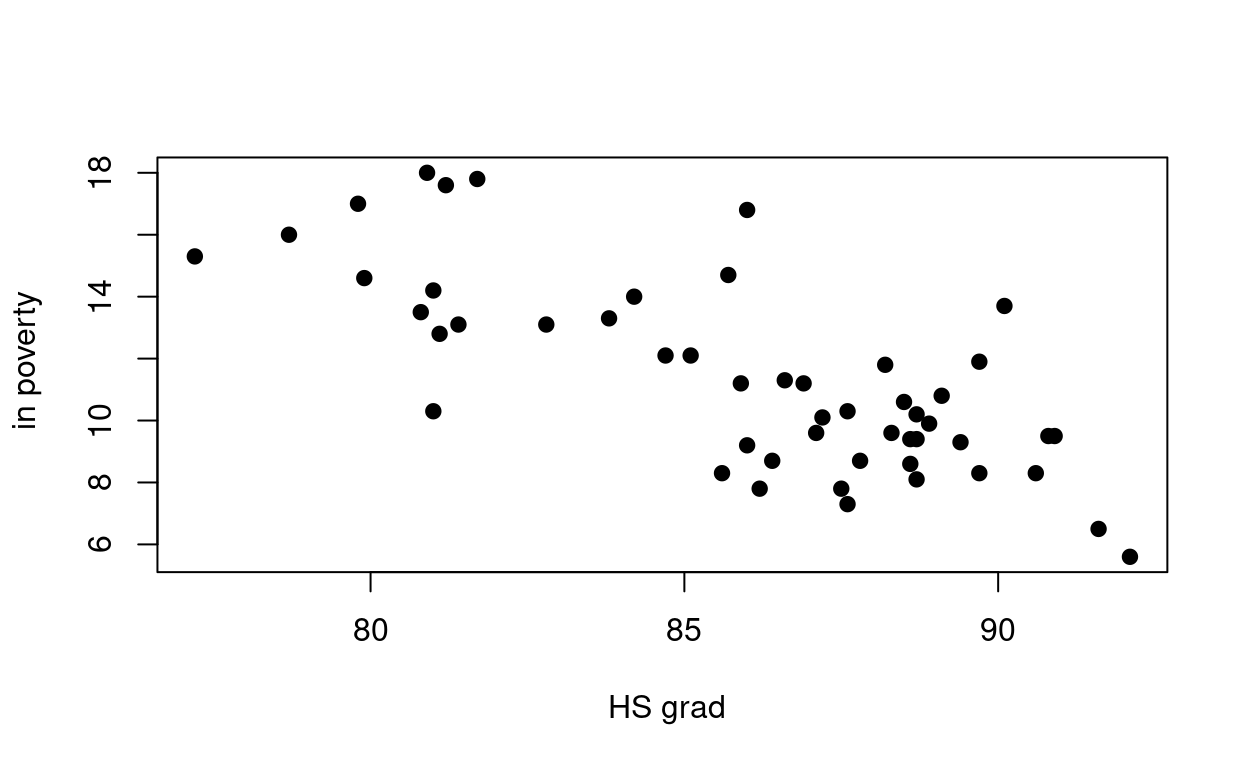
In the following equation:

\[Poverty = \beta_{0} - \beta_{1} \times Graduates + \epsilon\]

Based on the following model results:

## 
## Call:
## lm(formula = poverty$Poverty ~ poverty$Graduates)
## 
## Residuals:
##     Min      1Q  Median      3Q     Max 
## -4.1624 -1.2593 -0.2184  0.9611  5.4437 
## 
## Coefficients:
##                   Estimate Std. Error t value Pr(>|t|)    
## (Intercept)       64.78097    6.80260   9.523 9.94e-13 ***
## poverty$Graduates -0.62122    0.07902  -7.862 3.11e-10 ***
## ---
## Signif. codes:  0 '***' 0.001 '**' 0.01 '*' 0.05 '.' 0.1 ' ' 1
## 
## Residual standard error: 2.082 on 49 degrees of freedom
## Multiple R-squared:  0.5578, Adjusted R-squared:  0.5488 
## F-statistic: 61.81 on 1 and 49 DF,  p-value: 3.109e-10

Mathematical notations

We want to fit a line that has the smallest residuals:

\[RSS=\sum_{i=1}^{n}(y_i-\hat{y}_i)^2\]

In the above equation, \(\hat y\) stands for:

As you already know, A residual is the difference between the observed \(y_i\) and predicted \(\hat{y}_i\).

\[\epsilon_i = y_i - \hat{y}_i\] How far off will that single estimate of \(\hat{\mu}\) be?

• In general, we answer this question by computing the standard error of \(\hat{\mu}\), written as \(SE(\hat{\mu})\).

We have the well-known formula:

\[Var(\hat{\mu}) = SE(\hat{\mu})^2 = \frac{\sigma^2}{n}\]

So, the same way the standard deviation of a population is approximated by the standard error of sample:

As you know, TSS is the total sum of squares:

\[TSS = \sum_{i=1}^{n}(y_i - \bar{y})^2\]

Model accuracy

\(R^2\) is the proportion of variance explained. Here are some formulas:

1. \(R^2 = \frac{TSS - RSS}{TSS}\)
2. \(R^2 = 1 - \frac{RSE}{TSS}\)
3. \(R^2 = 1 - \frac{RSS}{TSS}\)
4. \(R^2 = 1 - \frac{TSS}{RSS}\)

Based on the following model results:

## 
## Call:
## lm(formula = poverty$Poverty ~ poverty$Graduates)
## 
## Residuals:
##     Min      1Q  Median      3Q     Max 
## -4.1624 -1.2593 -0.2184  0.9611  5.4437 
## 
## Coefficients:
##                   Estimate Std. Error t value Pr(>|t|)    
## (Intercept)       64.78097    6.80260   9.523 9.94e-13 ***
## poverty$Graduates -0.62122    0.07902  -7.862 3.11e-10 ***
## ---
## Signif. codes:  0 '***' 0.001 '**' 0.01 '*' 0.05 '.' 0.1 ' ' 1
## 
## Residual standard error: 2.082 on 49 degrees of freedom
## Multiple R-squared:  0.5578, Adjusted R-squared:  0.5488 
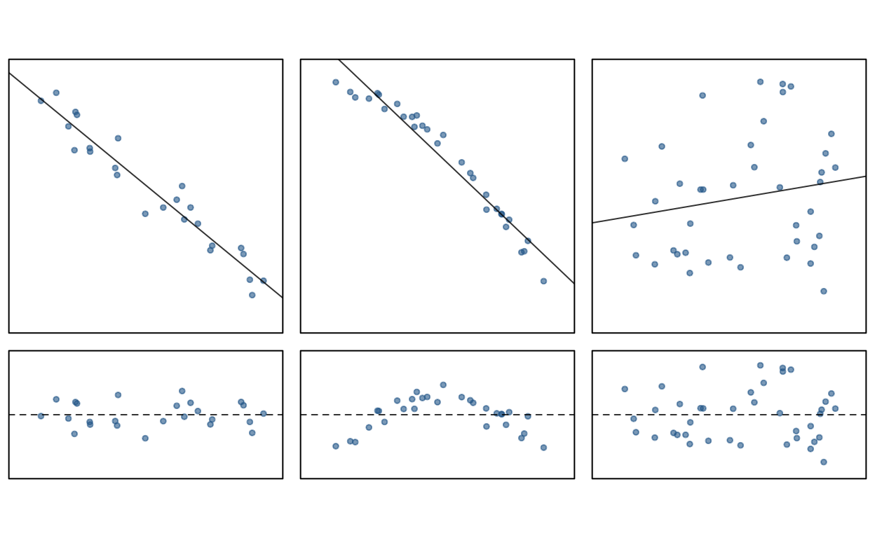
## F-statistic: 61.81 on 1 and 49 DF,  p-value: 3.109e-10

Model validity

Look at the following graph: