Regression analysis

Quadratic effects

A linear regression model was fit to predict how much money a customer would spend at an online retailer (in CAN$) based on the amount of time they were browsing the website (ranging between 1 and 100 minutes) along with the quadratic term for time. The coefficients table from the R output is:

	Estimate	SE	t-value	Pr(>|t|)
Intercept	6.902146	0.900384	7.666	9.41e-14	***
time	1.598175	0.122716	13.023	<2e-16	***
I(time^2)	-0.008558	0.002852	-3.001	0.00282	**

Binary & categorical independent variables

The main selling price of a sample of condos in Montreal was calculated to be $740,000 while the mean selling price of single family homes was calculated to the $975,000. If a regression mode was fit to predict selling price of a home based on a binary predictor for whether it was a condo ( x = 1 represents the condominium group).

Interactions

A regression model was fit to predict selling price of condos and single family homes in Montreal from \(x_1 = house~size\), \(x_2 =\) a binary independent variable for whether a home is a single family home (\(x_2 = 1\) for single family homes) and the interaction between the two. the estimated regression model is given below:

\[\hat y = 428 + 0.286 x_1 + 104 x_2 - 0.140 (x_1 \times x_2)\]

The regression model from the previous part is repeated here: to predict selling price of condominiums and single-family homes in Cambridge from x1 = house size, x2 = a binary predictor for whether a home is a single family home (x2 = 1 for single family homes), and the interaction between the two. The estimated regression model is given below:

\[\hat y = 428 + 0.286 x_1 + 104 x_2 - 0.140(x_1 \times x_2)\]

Comparing models

Two regression models are to be considered:

Model 1: \(y = \beta_0 + \beta_1 x_1\)

Model 2: \(y = \beta_0 + \beta_1 x_1 + \beta_2 x_2 + \beta_3 x_3\)

Two regression models are to be considered:

Model 1: \(y = \beta_0 + \beta_1 x_1\)

Model 2: \(y = \beta_0 + \beta_1 x_2 + \beta_2 x_3\)

Automatic Model Selection

Model diagnostics

You’d like to determine whether the normal distribution assumption is reasonable for a simple linear regression model.

Let us fit a linear regression:

re = read.csv("Real_Estate_Sample.csv")
lm1 = lm(Price ~ year, data=re)

The following histogram was produced after fitting the previous simple linear regression:

re = read.csv("Real_Estate_Sample.csv")
lm1 = lm(Price ~ year, data=re)

hist(lm1$residuals,col="gray")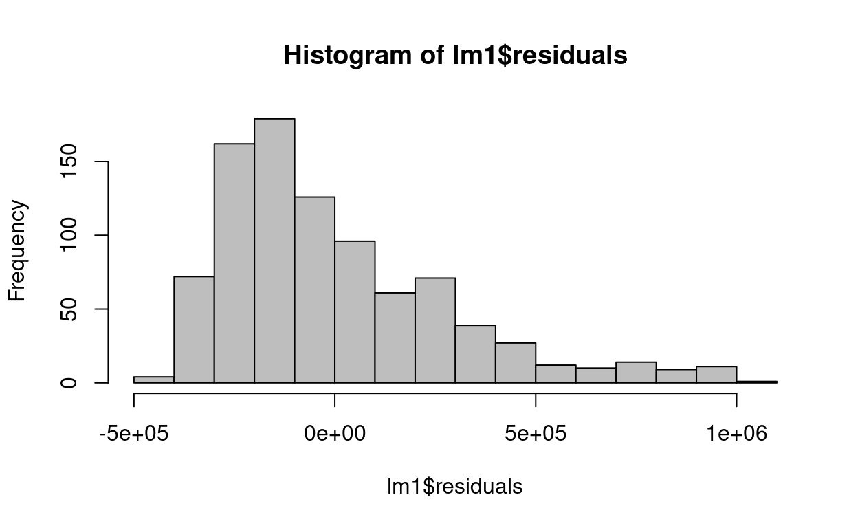

The following boxplot was produced after fitting a simple linear regression of Y on X:

boxplot(lm1$residuals,col="gray")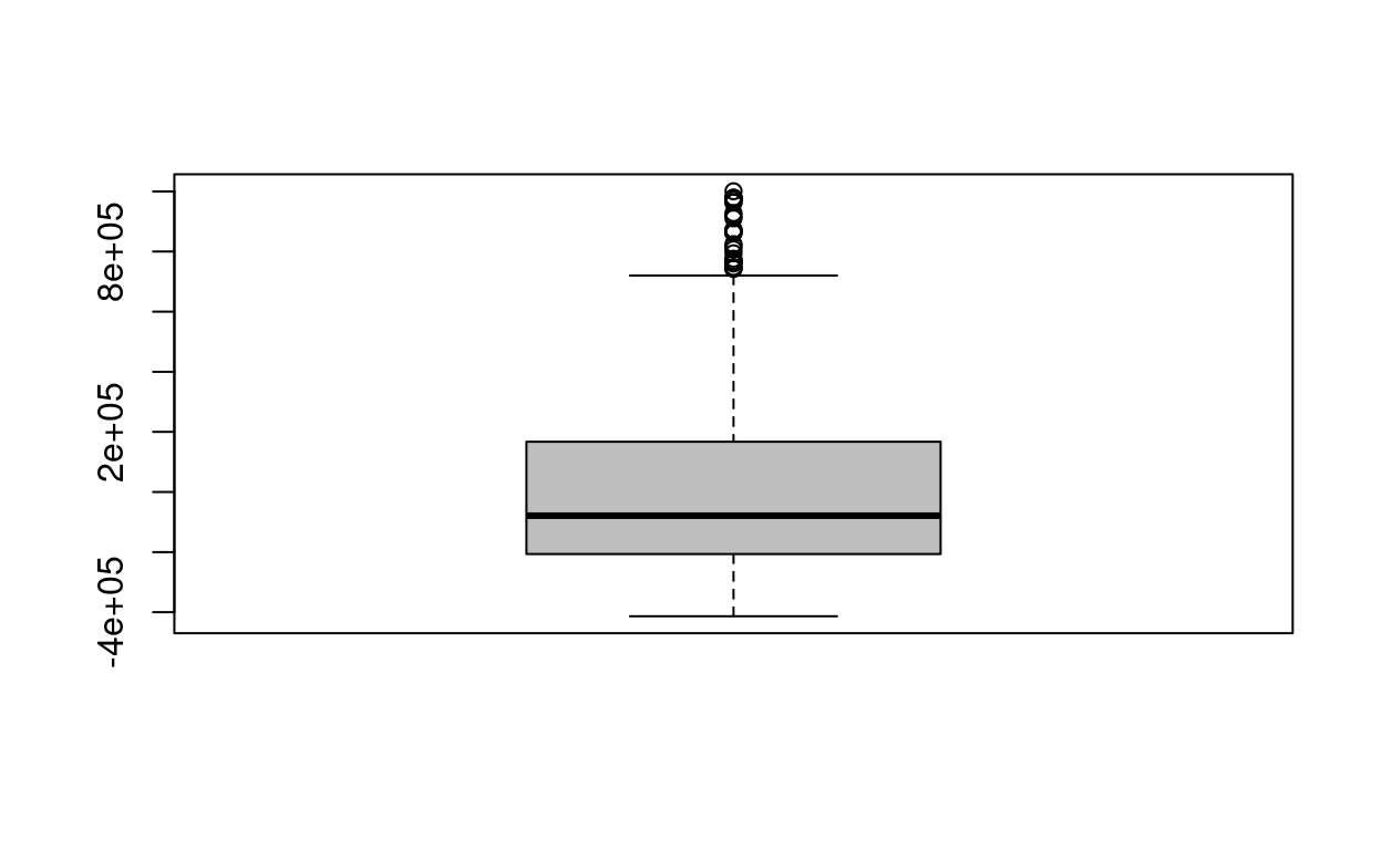

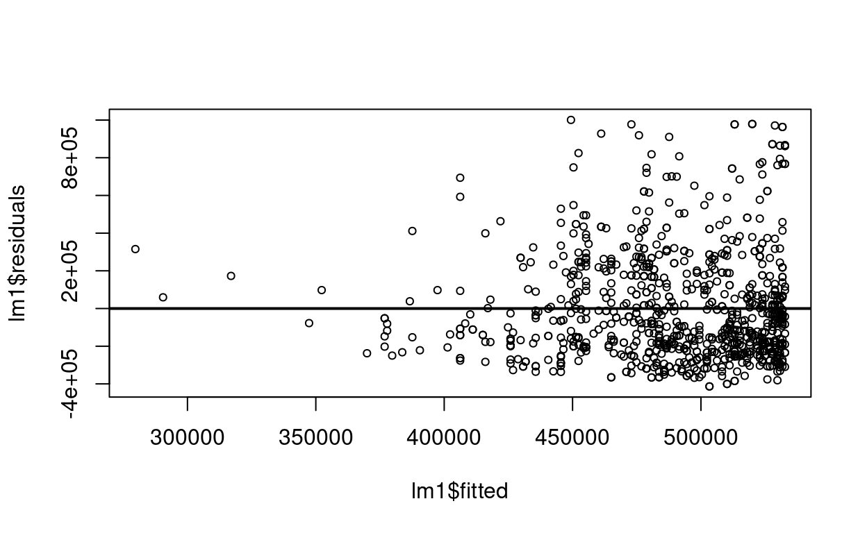
The following residual-versus-predicted scatterplot was produced after fitting a simple linear regression of Y on X:

plot(lm1$residuals~lm1$fitted,cex=0.7)
abline(h=0,lwd=2)