Introduction
This course is about using the power of computers to do things with geographic data. It teaches a range of spatial skills, including: reading, writing and manipulating geographic data; making static and interactive maps; applying geocomputation to solve real-world problems; and modeling geographic phenomena.
What is geocomputation?
Geocomputation is a young term, dating back to the first conference on the subject in 1996. What distinguished geocomputation from the (at the time) commonly used term ‘quantitative geography’, its early advocates proposed, was its emphasis on “creative and experimental” applications (Longley et al. 1998) and the development of new tools and methods (Openshaw and Abrahart 2000): “GeoComputation is about using the various different types of geodata and about developing relevant geo-tools within the overall context of a ‘scientific’ approach.”
Geocomputation is a recent term but is influenced by old ideas. It can be seen as a part of Geography, which has a 2000+ year history (Talbert 2014); and an extension of Geographic Information Systems (GIS) (Neteler and Mitasova 2008), which emerged in the 1960s (Coppock and Rhind 1991).
Geography has played an important role in explaining and influencing humanity’s relationship with the natural world long before the invention of the computer, however. Alexander von Humboldt’s travels to South America in the early 1800s illustrates this role: not only did the resulting observations lay the foundations for the traditions of physical and plant geography, they also paved the way towards policies to protect the natural world (Wulf 2015).
Why use R for geocomputation?
This ‘geodata revolution’ drives demand for high performance computer hardware and efficient, scalable software to handle and extract signal from the noise, to understand and perhaps change the world. Spatial databases enable storage and generation of manageable subsets from the vast geographic data stores, making interfaces for gaining knowledge from them vital tools for the future. R is one such tool, with advanced analysis, modeling and visualization capabilities.
In this context the focus of this course is not on the language itself. Instead we use R as a ‘tool for the trade’ for understanding the world, similar to Humboldt’s use of tools to gain a deep understanding of nature in all its complexity and interconnections. Although programming can seem like a reductionist activity, the aim is to teach geocomputation with R not only for fun, but for understanding the world.
R is a multi-platform, open source language and environment for statistical computing and graphics (r-project.org/). With a wide range of packages, R also supports advanced geospatial statistics, modeling and visualization. New integrated development environments (IDEs) such as RStudio have made R more user-friendly for many, easing map making with a panel dedicated to interactive visualization. Another example showing R’s flexibility and evolving geographic capabilities is interactive map making, as we’ll see in later sections.
Spatial Analysis
Motivation for using spatial analysis
Probably the most important argument for taking a spatial approach is that the independence assumption between observation is no longer valid. Attributes of observation i may influence the attributes of observation j.
To illustrate a very small set of what can be achieved in R for spatial analysis our running example will be examining violent crimes and foreclosures in the City of Chicago. The crime data as well as tracts shapefiles used here comes from Chicago Data Portal while foreclosures data come from the U.S. Department of Housing and Urban Development (HUD), all of these are public available.
R packages for spatial data analysis
In R, the fundamental unit of shareable code is the package. A package bundles together code, data, documentation, and tests, and is easy to share with others. As of April 2016, there were over 8,200 packages available on the Comprehensive R Archive Network, or CRAN, the public clearing house for R packages. This huge variety of packages is one of the reasons that R is so successful: the chances are that someone has already solved a problem that you’re working on, and you can benefit from their work by downloading their package. (Wickham (2015))
Spatial Analysis
R packages for spatial data analysis
Today we'll focus on using packages sf for handling spatial data, spdep for spatial dependencies, and leaflet for interactive mapping. To install these packages, type:
if(!requireNamespace("sf", quietly = TRUE)) {
  install.packages("sf")
}
if(!requireNamespace("spdep", quietly = TRUE)) {
  install.packages("spdep")
}
if(!requireNamespace("leaflet", quietly = TRUE)) {
  install.packages("leaflet")
}
if(!requireNamespace("RColorBrewer", quietly = TRUE)) {
  install.packages("RColorBrewer")
}
Now, we load the necessary libraries:
library(sf)
library(spdep)
library(leaflet)
Reading and Mapping spatial data in R
Spatial data comes in many "shapes" and "sizes", the most common types of spatial data are:
- Points are the most basic form of spatial data. Denotes a single point location, such as cities, a GPS reading or any other discrete object defined in space.
- Lines are a set of ordered points, connected by straight line segments
- Polygons denote an area, and can be thought as a sequence of connected points, where the first point is the same as the last
- Grid (Raster) are a collection of points or rectangular cells, organized in a regular lattice
For more details, see R. S. Bivand, Pebesma, and Gomez-Rubio (2008). Today we'll focus on Polygons. Spatial data usually comes in shapefile. This type of files stores non topological geometry and attribute information for the spatial features in a data set. Moreover, they don't require a lot of disk space and are easy to read and write. (ESRI (1998))
First we have to download and save the files in our computer from our server at http://www.econ.uiuc.edu/~lab/workshop/foreclosures/. I saved mine in my desktop. We've downloaded 3 files:
- Main file: foreclosures.shp
- Index file: foreclosures.shx
- dBASE table: foreclosures.dbf
The main file describes a shape with a list of its vertices. In the index file, each record contains the offset of the corresponding main file record from the beginning of the main file. The dBASE table contains feature attributes with one record per feature. (ESRI (1998))
To read data from a polygon shapefile into R we use the function st_read that will create a dataframe. To learn more about the function, the command ?st_read will give you access to the help file.
Spatial data in R can be easily managed using the sf package, which supports reading from various formats including shapefiles:
# Reading shapefiles using sf package
foreclosures_sf <- st_read('foreclosures.shp')
## Reading layer `foreclosures' from data source
## `/var/www/html/portfolio/shiny/mapping/foreclosures.shp' using driver `ESRI Shapefile'
## Simple feature collection with 897 features and 16 fields
## Geometry type: POLYGON
## Dimension: XY
## Bounding box: xmin: -87.94027 ymin: 41.64423 xmax: -87.52404 ymax: 42.03793
## CRS: NATo verify that the data has been read correctly and to see its structure, use:
print(foreclosures_sf)## Simple feature collection with 897 features and 16 fields
## Geometry type: POLYGON
## Dimension: XY
## Bounding box: xmin: -87.94027 ymin: 41.64423 xmax: -87.52404 ymax: 42.03793
## CRS: NA
## First 10 features:
## SP_ID fips est_fcs est_mtgs est_fcs_rt res_addr est_90d_va bls_unemp
## 1 1 17031010100 43 904 4.76 2530 12.61 8.16
## 2 2 17031010200 129 2122 6.08 3947 12.36 8.16
## 3 3 17031010300 55 1151 4.78 3204 10.46 8.16
## 4 4 17031010400 21 574 3.66 2306 5.03 8.16
## 5 5 17031010500 64 1427 4.48 5485 8.44 8.16
## 6 6 17031010600 56 1241 4.51 2994 6.58 8.16
## 7 7 17031010700 107 1959 5.46 3701 5.78 8.16
## 8 8 17031010800 43 830 5.18 1694 6.91 8.16
## 9 9 17031010900 7 208 3.37 443 9.93 8.16
## 10 10 17031020100 51 928 5.50 1552 7.15 8.16
## county fips_num totpop tothu huage oomedval property violent
## 1 Cook County 17031010100 5391 2557 61 169900 646 433
## 2 Cook County 17031010200 10706 3981 53 147000 914 421
## 3 Cook County 17031010300 6649 3281 56 119800 478 235
## 4 Cook County 17031010400 5325 2464 60 151500 509 159
## 5 Cook County 17031010500 10944 5843 54 143600 641 240
## 6 Cook County 17031010600 7178 3136 58 145900 612 266
## 7 Cook County 17031010700 10799 3875 48 153400 678 272
## 8 Cook County 17031010800 5403 1768 57 170500 332 146
## 9 Cook County 17031010900 1089 453 61 215900 147 78
## 10 Cook County 17031020100 3634 1555 48 114700 351 84
## geometry
## 1 POLYGON ((-87.67736 42.0230...
## 2 POLYGON ((-87.67326 42.0192...
## 3 POLYGON ((-87.66866 42.0194...
## 4 POLYGON ((-87.66251 42.0128...
## 5 POLYGON ((-87.66372 42.0127...
## 6 POLYGON ((-87.66578 42.0128...
## 7 POLYGON ((-87.67056 42.0127...
## 8 POLYGON ((-87.67096 42.0054...
## 9 POLYGON ((-87.66856 42.0036...
## 10 POLYGON ((-87.68496 42.0194...class(foreclosures_sf)## [1] "sf" "data.frame"You can plot the spatial data using base plot functions or using ggplot2:
plot(foreclosures_sf)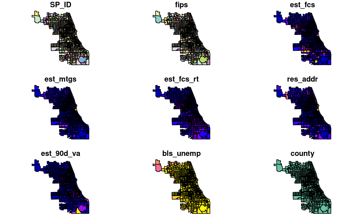
For interactive mapping, you can directly use foreclosures_sf with the leaflet package:
library(leaflet)

leaflet(foreclosures_sf) %>%
  addTiles() %>%
  addPolygons(stroke = FALSE, fillOpacity = 0.5, smoothFactor = 0.5)
Mapping with Leaflet
Basic Usage
You create a Leaflet map with these basic steps:
- Create a map widget by calling leaflet().
- Add layers (i.e., features) to the map by using layer functions (e.g. addTiles, addMarkers, addPolygons) to modify the map widget.
- Repeat step 2 as desired.
- Print the map widget to display it.
library(leaflet)Without Marker
leaflet() %>%
  setView(lng = -73.582189, lat = 45.517958, zoom = 14) %>%
  addTiles()
With Marker
leaflet() %>%
  addTiles() %>%
  addMarkers(lng=-73.582189, lat=45.517958, popup="The birthplace of Nüance-R")
Data Object
Both leaflet() and the map layer functions have an optional data parameter that is designed to receive spatial data in one of several forms:
- From base R:
- lng/lat matrix
- data frame with lng/lat columns
- From the sp package: -SpatialPoints[DataFrame]
- Line/Lines
- SpatialLines[DataFrame]
- Polygon/Polygons
- SpatialPolygons[DataFrame]
- From the maps package:
- the data frame from returned from map()
Here an example with our data seen in the previous section.
library(leaflet)
leaflet(foreclosures_sf) %>%
  addPolygons(stroke = FALSE, fillOpacity = 0.5, smoothFactor = 0.5) %>%
  addTiles() #adds a map tile, the default is OpenStreetMap
we can add color using the package RColorBrewer
require(RColorBrewer)qpal<-colorQuantile("OrRd", foreclosures_sf$violent, n=9)
leaflet(foreclosures_sf) %>%
addPolygons(stroke = FALSE, fillOpacity = .8, smoothFactor = 0.2, color = ~qpal(violent)) %>%
addTiles()The colorQuantile function of the leaflet package maps values of the data to colors following a palette. In this case I've specified a palette of Oranges and Reds, for more palettes you can access the help file for RColorBrewer: ?RColorBrewer.
Spatial Econometrics
When dealing with space one must bear in mind Tobler’s first law of geography “Everything is related to everything else, but close things are more related than things that are far apart”(Tobler (1979)). In this section we’ll focus on the specification of spatial dependence, on specification tests to detect spatial dependence in regressions models and on basic regression models that incorporate spatial dependence. We’ll illustrate this using the data in the shapefile loaded in the previous section.
OLS regression
The traditional approach for many years has been to ignore the spatial dependence of the data and just run an OLS regression.
\[y = X \beta + \epsilon\]
In R this is achieved with the lm function. For example,
chi.ols<-lm(violent ~ est_fcs_rt + bls_unemp, data=foreclosures_sf)I’ve specified the “model” as violent~est_fcs_rt+bls_unemp where violent is the dependent variable and, est_fcs_rt and bls_unemp are the explanatory variable. I’ve also specified the data set which is the slot data of our shapefile. Note that to access this slot I use the @ symbol. This line does not return anything because we have created an lm object that I called chi.ols. To see the results, we use the summary function
summary(chi.ols)##
## Call:
## lm(formula = violent ~ est_fcs_rt + bls_unemp, data = foreclosures_sf)
##
## Residuals:
## Min 1Q Median 3Q Max
## -892.02 -77.02 -23.73 41.90 1238.22
##
## Coefficients:
## Estimate Std. Error t value Pr(>|t|)
## (Intercept) -18.627 45.366 -0.411 0.681
## est_fcs_rt 28.298 1.435 19.720 <2e-16 ***
## bls_unemp -0.308 5.770 -0.053 0.957
## ---
## Signif. codes: 0 '***' 0.001 '**' 0.01 '*' 0.05 '.' 0.1 ' ' 1
##
## Residual standard error: 157.3 on 894 degrees of freedom
## Multiple R-squared: 0.3141, Adjusted R-squared: 0.3126
## F-statistic: 204.7 on 2 and 894 DF, p-value: < 2.2e-16The problem with ignoring the spatial structure of the data implies that the OLS estimates in the non spatial model may be biased, inconsistent or inefficient, depending on what is the true underlying dependence (for more see Anselin and Bera (1998)).
Modeling Spatial Dependence
We now take a closer look at spatial dependence, or to be more precise on it’s weaker expression spatial autocorrelation. Spatial autocorrelation measures the degree to which a phenomenon of interest is correlated to itself in space (Cliff and Ord (1973)). In other words, similar values appear close to each other, or cluster, in space (positive spatial autocorrelation) or neighboring values are dissimilar (negative spatial autocorrelation). Null spatial autocorrelation indicates that the spatial pattern is random. Following Anselin and Bera (1998) we can express the existence of spatial autocorrelation with the following moment condition:
\[Cov(y_{i},y_{j})\neq 0\,\,\,\, for\,\,\,\,i\neq j\]
where \(Cov(y_{i},y_{j})\) is the covariance between two observations
were yi and yj are observations on a random variable at locations i and j. The problem here is that we need to estimate N by N covariance terms directly for N observations. To overcome this problem we impose restrictions on the nature of the interactions. One type of restriction is to define for each data point a relevant "neighborhood set". In spatial econometrics this is operationalized via the spatial weights matrix. The matrix usually denoted by W is a N by N positive and symmetric matrix which denotes fore each observation (row) those locations (columns) that belong to its neighborhood set as nonzero elements (Anselin and Bera (1998), Arbia (2014)), the typical element is then:
\[[w_{ij}]=\begin{cases} 1 & if\,j\in N\left(i\right) \\ 0 & o.w \end{cases}\]
where \(N\left(i\right)\) is the neighborhood set of location i and N(i) being the set of neighbors of location j. By convention, the diagonal elements are set to zero, i.e. \(w_{ii} = 0\). To help with the interpretation the matrix is often row standardized such that the elements of a given row add to one.
The specification of the neighboring set is quite arbitrary and there's a wide range of suggestions in the literature. One popular way is to use one of the two following criteria:
- Rook criterion: two units are close to one another if they share a side
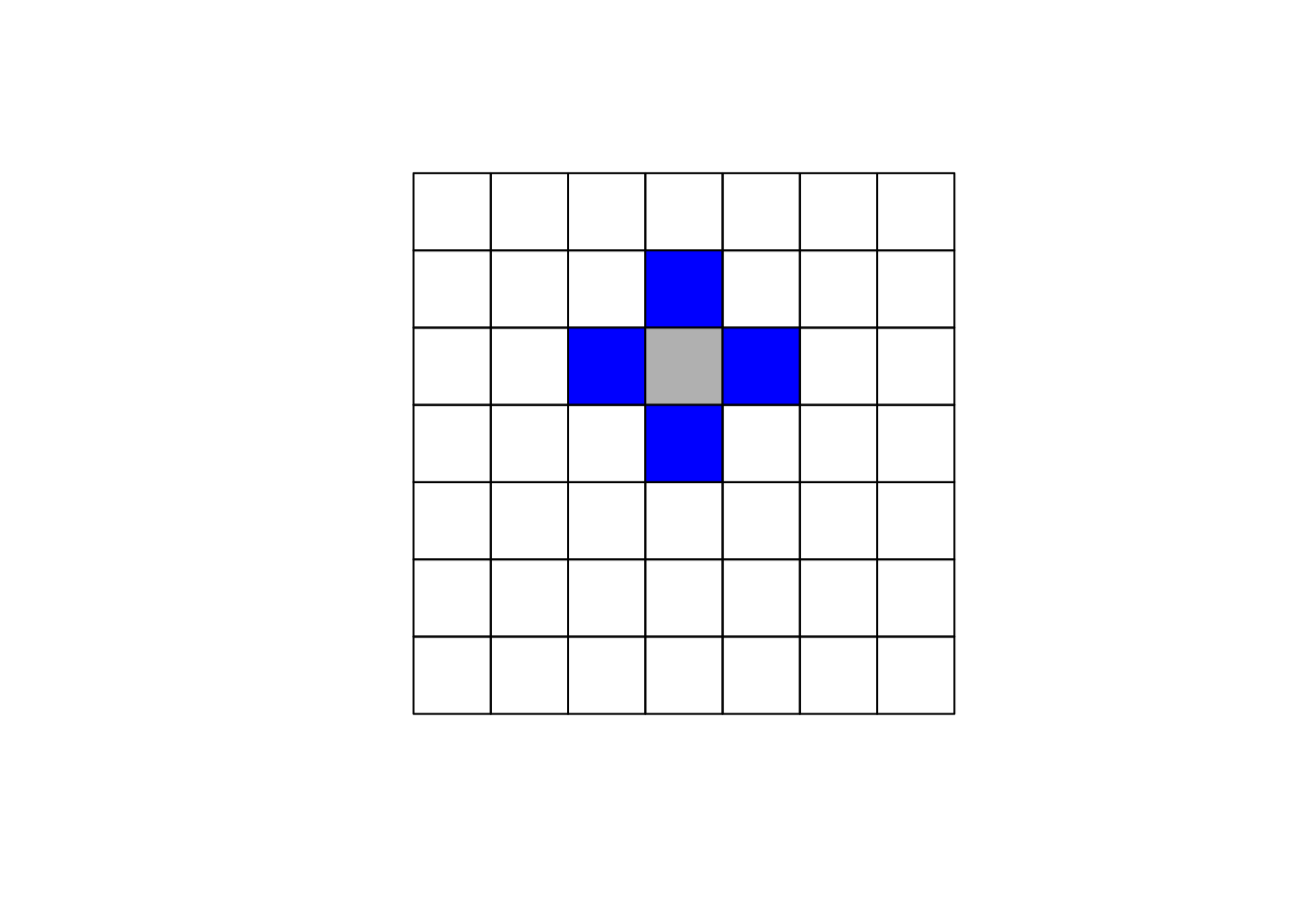
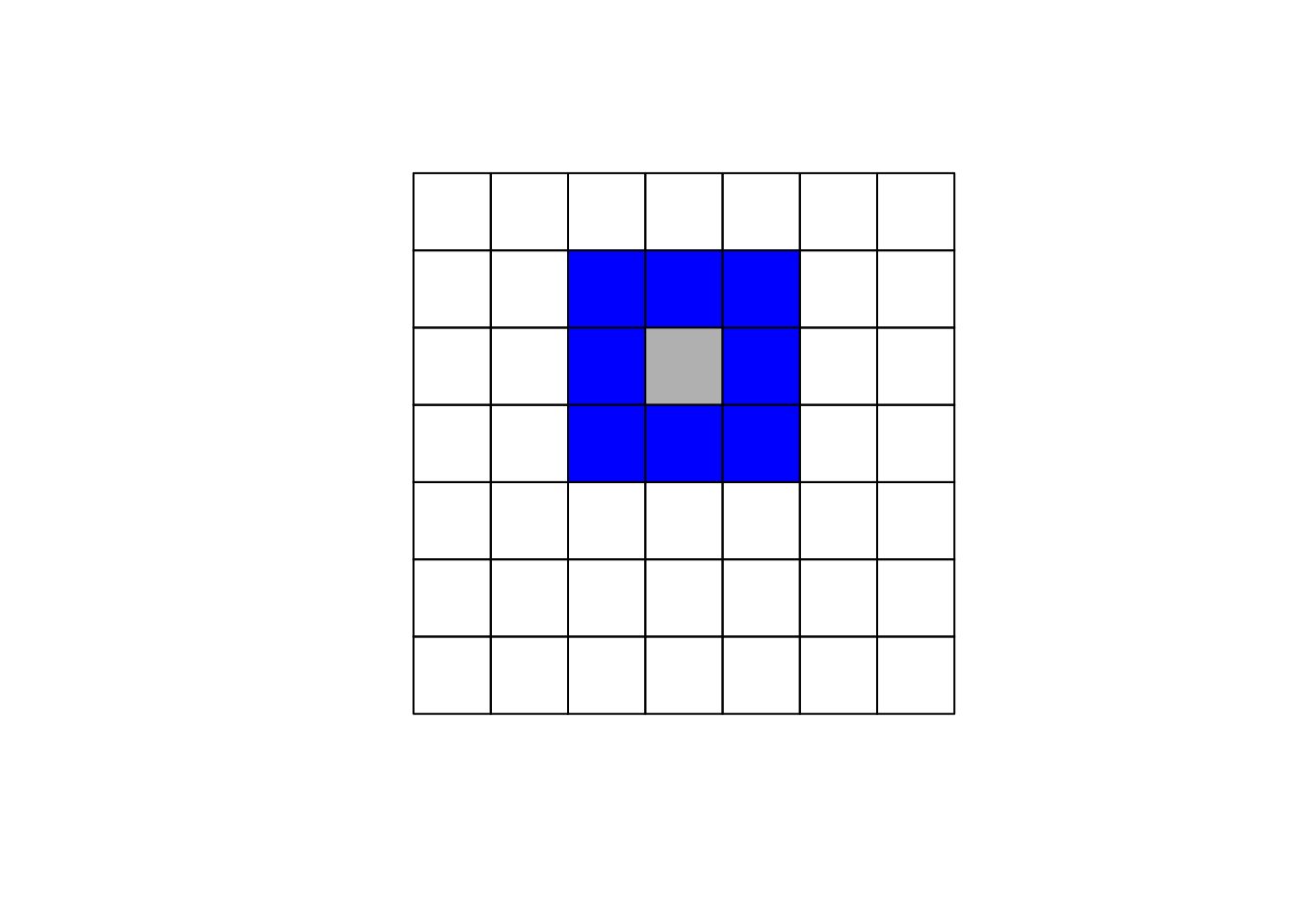
- Queen criterion: two units are close if they share a side or an edge.
Another used approach is to denote two observations as neighbors if they are within a certain distance, i.e., \(j\) \(\in N\left(j\right)\) if \(d_{ij} < d_{max}\) where \(d\) is the distance between location \(i\) and \(j\) .
Here we'll focus on using the queen criterion and we encourage the reader to experiment with the rook criterion. In R to obtain the weights matrix we make use of two functions. In the first step we use poly2nb which builds a neighbors list, if the option queen=TRUE is specified it will be build using the queen criterion. If FALSE is specified, then the rook criteria will be used. The next step is to supplement the neighbors list with the spatial weights. The option W row standardizes the matrix.
# Ensure spdep is loaded for spatial dependency features
library(spdep)

# Create neighbors using poly2nb, which now supports sf objects directly
neighbors <- poly2nb(foreclosures_sf, queen=TRUE)

# Create a listw object from the neighbors
W <- nb2listw(neighbors, style="W", zero.policy=TRUE)
We can plot the link distribution with the usual plot function
library(leaflet)
leaflet(foreclosures_sf) %>%
 # addProviderTiles(providers$OpenStreetMap) %>%
  addPolygons(fillColor = ~ifelse(as.character(1:nrow(foreclosures_sf)) %in% names(unlist(neighbors)), "#FF7777", "#7777FF"),
              color = "#FFFFFF",
              fillOpacity = 0.7,
              popup = ~paste("ID:", row.names(foreclosures_sf))) %>%
  addLegend(position = "bottomright",
            values = ~ifelse(as.character(1:nrow(foreclosures_sf)) %in% names(unlist(neighbors)), "Neighbor", "Non-neighbor"),
            title = "Legend",
            colors = c("#FF7777", "#7777FF"),  # Define colors corresponding to the values
            labels = c("Neighbor", "Non-neighbor"),
            opacity = 1.0)
To obtain the weight matrix based on distances we use two functions: coordinates that will retrieve the centroid coordinates of the census tracts polygons and dnearneigh that will identify neighbors between two distances in kilometers measured using Euclidean distance. For example, to find neighbors within 1 kilometer we do:
library(sf)
library(spdep)

# Assuming foreclosures_sf is already loaded as an 'sf' object

# Calculate centroids of the geometries
centroids <- st_centroid(foreclosures_sf)

# Extract coordinates from the centroids
coords <- st_coordinates(centroids)

# Check the dimensions to ensure it's correct for dnearneigh()
print(dim(coords))  # Should print a two-column matrix
## [1] 897 2# Create a neighbors list based on distance (e.g., neighbors within 1 kilometer)
# Ensure the units are appropriate for the CRS of your data
W_dist <- dnearneigh(coords, 0, 1, longlat = FALSE)
# If you need to convert this neighbors list to a weights list
W_dist_weights <- nb2listw(W_dist, style = "W", zero.policy = TRUE)I encourage you to compare the link distributions for these three ways of defining neighbors.
Spatial Autoregressive (SAR) Models
Spatial lag dependence in a regression setting can be modeled similar to an autoregressive process in time series. Formally, \[y=\rho Wy+X \beta+\epsilon\] The presence of the term \(Wy\) induces a nonzero correlation with the error term, similar to the presence of an endogenous variable, but different from the time series context. Contrarious to time series, \([Wy]_i\) is always correlated with \(\epsilon\) irrespective of the structure of the errors. This implies that OLS estimates in the non spatial model will be biased and inconsistent. (Anselin and Bera (1998))
Spatial Error Models (SEM)
Another way to model spatial autocorrelation in a regression model is to specify the autoregressive process in the error term: \[ y=X \beta+\epsilon \] with \[\epsilon=\lambda W \epsilon+u\] If this is the "true" form of spatial dependence OLS estimates will be unbiased but inefficient. Testing for spatial autocorrelation
Testing for spatial autocorrelation
There are multiple tests for testing the presence of spatial autocorrelation. In this note we'll focus on a restricted set: Moran's I test and Lagrange Multiplier tests.
Moran's I Test
Moran's I test was originally developed as a two-dimensional analog of Durbin-Watson's test
\[I = \left( \frac{e'We}{e'e} \right)\]
where \(e = y − X\beta\) is a vector of OLS residuals, \(\beta = (X'X)^{-1} X'y\), \(W\) is the row standardized spatial weights matrix.(For more detail see Anselin and Bera (1998)) To perform a Moran test on our data we need two inputs, an lm regression object (estimated in the OLS section) and the spatial weight matrix
moran.lm <- lm.morantest(chi.ols, W, alternative="two.sided")
print(moran.lm)
##
## Global Moran I for regression residuals
##
## data:
## model: lm(formula = violent ~ est_fcs_rt + bls_unemp, data =
## foreclosures_sf)
## weights: W
##
## Moran I statistic standard deviate = 11.785, p-value < 2.2e-16
## alternative hypothesis: two.sided
## sample estimates:
## Observed Moran I Expectation Variance
## 0.2142252370 -0.0020099108 0.0003366648The computation of the statistic is relative to a given choice of the spatial weights W. Different specifications of the weights matrix will give different results. I encourage the reader to try this with the rook contiguity criterion.
Lagrange Multiplier Test
A nice feature of Moran's I test is that i has high power against a wide range of alternatives (Anselin and Bera (1998)). However, it does not guide us in the selection of alternative models. On the other hand, Lagrange Multiplier test specify the alternative hypothesis which will help us with the task. The LM tests for spatial dependence are included in the lm.LMtests function and include as alternatives the presence of a spatial lag and the presence of a spatial lag in the error term. Both tests, as well as their robust forms are included in the lm.LMtests function. To call them we use the option test="all". Again, a regression object and a spatial listw object must be passed as arguments:
LM <- lm.LMtests(chi.ols, W, test="all")
print(LM)
##
## Rao's score (a.k.a Lagrange multiplier) diagnostics for spatial
## dependence
##
## data:
## model: lm(formula = violent ~ est_fcs_rt + bls_unemp, data =
## foreclosures_sf)
## test weights: listw
##
## RSerr = 134.52, df = 1, p-value < 2.2e-16
##
##
## Rao's score (a.k.a Lagrange multiplier) diagnostics for spatial
## dependence
##
## data:
## model: lm(formula = violent ~ est_fcs_rt + bls_unemp, data =
## foreclosures_sf)
## test weights: listw
##
## RSlag = 182.18, df = 1, p-value < 2.2e-16
##
##
## Rao's score (a.k.a Lagrange multiplier) diagnostics for spatial
## dependence
##
## data:
## model: lm(formula = violent ~ est_fcs_rt + bls_unemp, data =
## foreclosures_sf)
## test weights: listw
##
## adjRSerr = 0.00066762, df = 1, p-value = 0.9794
##
##
## Rao's score (a.k.a Lagrange multiplier) diagnostics for spatial
## dependence
##
## data:
## model: lm(formula = violent ~ est_fcs_rt + bls_unemp, data =
## foreclosures_sf)
## test weights: listw
##
## adjRSlag = 47.653, df = 1, p-value = 5.089e-12
##
##
## Rao's score (a.k.a Lagrange multiplier) diagnostics for spatial
## dependence
##
## data:
## model: lm(formula = violent ~ est_fcs_rt + bls_unemp, data =
## foreclosures_sf)
## test weights: listw
##
## SARMA = 182.18, df = 2, p-value < 2.2e-16Since LMerr and LMlag are both statistically significant different from zero, we need to look at their robust counterparts. These robust counterparts are actually robust to the presence of the other "type" of autocorrelation. The robust version of the tests suggest that the lag model is the more likely alternative.
Running Spatial Regressions
SAR Models
The estimation of the SAR model can be approached in two ways. One way is to assume normality of the error term and use maximum likelihood. This is achieved in R with the function lagsarlm
if (!requireNamespace("spatialreg", quietly = TRUE)) {
    install.packages("spatialreg")
}
library(spatialreg)

sar.chi <- lagsarlm(violent ~ est_fcs_rt + bls_unemp, data = foreclosures_sf, W)
summary(sar.chi)
##
## Call:
## lagsarlm(formula = violent ~ est_fcs_rt + bls_unemp, data = foreclosures_sf,
## listw = W)
##
## Residuals:
## Min 1Q Median 3Q Max
## -519.127 -65.003 -15.226 36.423 1184.193
##
## Type: lag
## Coefficients: (asymptotic standard errors)
## Estimate Std. Error z value Pr(>|z|)
## (Intercept) -93.7885 41.3162 -2.270 0.02321
## est_fcs_rt 15.6822 1.5600 10.053 < 2e-16
## bls_unemp 8.8949 5.2447 1.696 0.08989
##
## Rho: 0.49037, LR test value: 141.33, p-value: < 2.22e-16
## Asymptotic standard error: 0.039524
## z-value: 12.407, p-value: < 2.22e-16
## Wald statistic: 153.93, p-value: < 2.22e-16
##
## Log likelihood: -5738.047 for lag model
## ML residual variance (sigma squared): 20200, (sigma: 142.13)
## Number of observations: 897
## Number of parameters estimated: 5
## AIC: 11486, (AIC for lm: 11625)
## LM test for residual autocorrelation
## test value: 8.1464, p-value: 0.0043146Another way is to use 2SLS using the function stsls. I leave this to the reader so he/she can compare the results to the MLE approach. The function is:
sar2sls.chi<-stsls(violent ~ est_fcs_rt + bls_unemp, data = foreclosures_sf, W)
summary(sar2sls.chi)
##
## Call:stsls(formula = violent ~ est_fcs_rt + bls_unemp, data = foreclosures_sf,
## listw = W)
##
## Residuals:
## Min 1Q Median 3Q Max
## -472.703 -61.955 -12.668 36.795 1168.899
##
## Coefficients:
## Estimate Std. Error t value Pr(>|t|)
## Rho 0.629161 0.082777 7.6007 2.953e-14
## (Intercept) -115.062608 42.648091 -2.6980 0.006977
## est_fcs_rt 12.111383 2.488729 4.8665 1.136e-06
## bls_unemp 11.499706 5.406927 2.1268 0.033433
##
## Residual variance (sigma squared): 19943, (sigma: 141.22)
## Anselin-Kelejian (1997) test for residual autocorrelation
## test value: 6.1515, p-value: 0.01313We then can compare the residuals of the OLS regression to the residuals of the spatial autoregressive model. To access the residuals for the OLS model and the SAR model we simply do
library(ggplot2)
library(sf)

# Assuming the residuals are correctly in foreclosures_sf
foreclosures_sf$chi.sar.res <- resid(sar.chi)

# Plot using ggplot2
ggplot(foreclosures_sf) +
  geom_sf(aes(fill = chi.sar.res)) +
  scale_fill_gradientn(colors = rev(brewer.pal(11, "RdBu"))) +
  theme_minimal()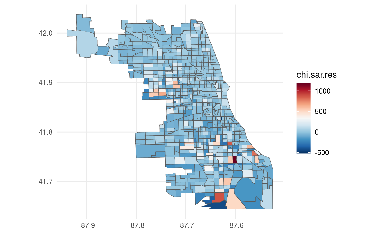
library(ggplot2)
library(sf)

# Assuming the residuals are correctly in foreclosures_sf
foreclosures_sf$chi.ols.res <- resid(chi.ols)

# Plot using ggplot2
ggplot(foreclosures_sf) +
  geom_sf(aes(fill = chi.ols.res)) +
  scale_fill_gradientn(colors = rev(brewer.pal(11, "RdBu"))) +
  theme_minimal()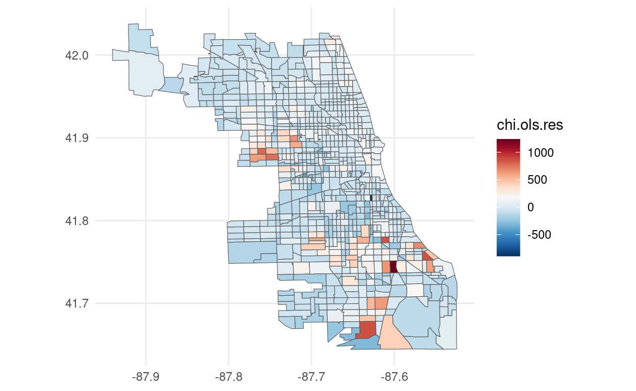
Marginal Effects
Note that the presence of the spatial weights matrix makes marginal effects richer and slightly more complicated than in the "traditional" OLS model. We'll have three impact measures suggested by Pace and LeSage (2009) and is done in R with the function impacts
impacts(sar.chi, listw = W)## Impact measures (lag, exact):
## Direct Indirect Total
## est_fcs_rt dy/dx 16.434478 14.336896 30.77137
## bls_unemp dy/dx 9.321585 8.131843 17.45343The direct impact refers to average total impact of a change of an independent variable on the dependent fore each observation, i.e., \(n^{-1}\sum_{i=1}^n\frac{\partial E\left(y_i\right)}{\partial X_i}\) the indirect impact which is the sum of the impact produced on one single observation by all other observations and the impact of one observation on all the other. The total is the summation of the two
SEM Models
On the other hand, if we want to estimate the Spatial Error Model we have two approaches again. First, we can use Maximum Likelihood as before, with the function errorsarlm
errorsalm.chi <- errorsarlm(violent ~ est_fcs_rt + bls_unemp, data = foreclosures_sf, W)
summary(errorsalm.chi)
##
## Call:
## errorsarlm(formula = violent ~ est_fcs_rt + bls_unemp, data = foreclosures_sf,
## listw = W)
##
## Residuals:
## Min 1Q Median 3Q Max
## -650.506 -64.355 -22.646 35.461 1206.346
##
## Type: error
## Coefficients: (asymptotic standard errors)
## Estimate Std. Error z value Pr(>|z|)
## (Intercept) -1.2624 43.0509 -0.0293 0.9766
## est_fcs_rt 19.4620 1.9450 10.0062 <2e-16
## bls_unemp 4.0380 5.5134 0.7324 0.4639
##
## Lambda: 0.52056, LR test value: 109.68, p-value: < 2.22e-16
## Asymptotic standard error: 0.042291
## z-value: 12.309, p-value: < 2.22e-16
## Wald statistic: 151.51, p-value: < 2.22e-16
##
## Log likelihood: -5753.875 for error model
## ML residual variance (sigma squared): 20796, (sigma: 144.21)
## Number of observations: 897
## Number of parameters estimated: 5
## AIC: 11518, (AIC for lm: 11625)The same plot for the SEM residuals can be done as before and is left for the reader. A second approach is use Feasible Generalized Least Squares (GLS) with the function GMerrorsar. The function is:
fgls.chi <- GMerrorsar(violent ~ est_fcs_rt + bls_unemp, data= foreclosures_sf, W)
summary(fgls.chi)
##
## Call:
## GMerrorsar(formula = violent ~ est_fcs_rt + bls_unemp, data = foreclosures_sf,
## listw = W)
##
## Residuals:
## Min 1Q Median 3Q Max
## -697.623 -76.205 -33.292 44.053 1271.737
##
## Type: GM SAR estimator
## Coefficients: (GM standard errors)
## Estimate Std. Error z value Pr(>|z|)
## (Intercept) -1.8587 43.5671 -0.0427 0.9660
## est_fcs_rt 21.1757 1.8752 11.2925 <2e-16
## bls_unemp 2.9037 5.5869 0.5197 0.6032
##
## Lambda: 0.44789 (standard error): 0.11067 (z-value): 4.0473
## Residual variance (sigma squared): 21515, (sigma: 146.68)
## GM argmin sigma squared: 21607
## Number of observations: 897
## Number of parameters estimated: 5Finally, if we look at the likelihood for the SAR model and SEM model we see that we achieve a lower value for the SAR model that was the model favored by the LMtests. The residuals plot presented above still show some presence of spatial autocorrelation. It's very likely that the a more complete model is specified. The literature has expanded to more complex models. The reader is encouraged to read Anselin and Bera (1998), Arbia (2014) and Pace and LeSage (2009) for more detailed and complete introductions on Spatial Econometrics.
References
Anselin, Luc. 2003. “An Introduction to Spatial Regression Analysis in R.” Available at: Https://Geodacenter.asu.edu/Drupal\_files/Spdepintro.pdf.
Anselin, Luc, and Anil K Bera. 1998. “Spatial Dependence in Linear Regression Models with an Introduction to Spatial Econometrics.” Statistics Textbooks and Monographs 155. MARCEL DEKKER AG: 237–90.
Arbia, Giuseppe. 2014. A Primer for Spatial Econometrics: With Applications in R. Palgrave Macmillan.
Bivand, Roger S, Edzer J Pebesma, and Virgilio Gomez-Rubio. 2008. Applied Spatial Data Analysis with R. Springer. Springer.
Bivand, Roger, and Nicholas Lewin-Koh. 2016. Maptools: Tools for Reading and Handling Spatial Objects. https://CRAN.R-project.org/package=maptools.
Bivand, Roger, and Gianfranco Piras. 2015. “Comparing Implementations of Estimation Methods for Spatial Econometrics.” Journal of Statistical Software 63. 18.: 1–36. http://www.jstatsoft.org/v63/i18/.
Bivand, Roger, Jan Hauke, and Tomasz Kossowski. 2013. “Computing the Jacobian in Gaussian Spatial Autoregressive Models: An Illustrated Comparison of Available Methods.” Geographical Analysis 45. 2.: 150–79. http://www.jstatsoft.org/v63/i18/.
Cheng, Joe, and Yihui Xie. 2015. Leaflet: Create Interactive Web Maps with the Javascript ’Leaflet’ Library. http://rstudio.github.io/leaflet/.
Cliff, Andrew David, and J Keith Ord. 1973. Spatial Autocorrelation. Vol. 5. Pion London.
ESRI, Environmental Systems Research Institute. 1998. “ESRI Shapefile Technical Description.” Available at: Https://Www.esri.com/Library/Whitepapers/Pdfs/Shapefile.pdf.
Neuwirth, Erich. 2014. RColorBrewer: ColorBrewer Palettes. https://CRAN.R-project.org/package=RColorBrewer.
Pace, R Kelley, and JP LeSage. 2009. “Introduction to Spatial Econometrics.” Boca Raton, FL: Chapman &Hall/CRC.
Tobler, WR. 1979. “Cellular Geography.” In Philosophy in Geography, 379–86. Springer.
Wickham, Hadley. 2015. R Packages. “O’Reilly Media, Inc.”
Acknowledgments
To cite this course:
```
Notes
- The
sfpackage functions are used for reading and handling spatial data, replacing the oldermaptoolsandsppackage functions. - The
st_read()function fromsfis used to read shapefiles directly into ansfobject, which is more efficient and integrates well with modern R practices, includingdplyrandggplot2. - You might need to adjust subsequent code depending on how the spatial data is handled and analyzed, especially if specific
maptoolsfunctionalities were previously used that have directsfequivalents.
This updated script will keep your course content modern and compatible with the latest tools and practices in R for spatial data analysis.
Warin, Thierry. 2020. “Covid-19 Simulation: A Data Science Perspective.” doi:10.6084/m9.figshare.12020994.v1.