Introduction
In this first laboratory, you will familiarize yourself with the environment used for this course. All research projects are made with RStudio, an integrated development environment using the R programming language as well as Markdown. The goal of this course is to harness the power of data science tools for international business. In this regard, we promote reproducible research as our research method. In order to do so, RStudio, with documents written in Markdown, will be your main portal for doing your projects. You will learn a few syntax tips regarding Markdown and how to save your projects online (Git). Throughout the laboratory, useful tips will be either displayed in bold or in italics.
Goals
At the end of the lab, you should be able to:
- familiarize with the RStudio Integrated Development Environment
- create your first document in RStudio
- understand the Markdown syntax and knit your document
- synchronize your project with Git
Keywords: RStudio; Markdown; Git; reproducible research
RStudio
Environment
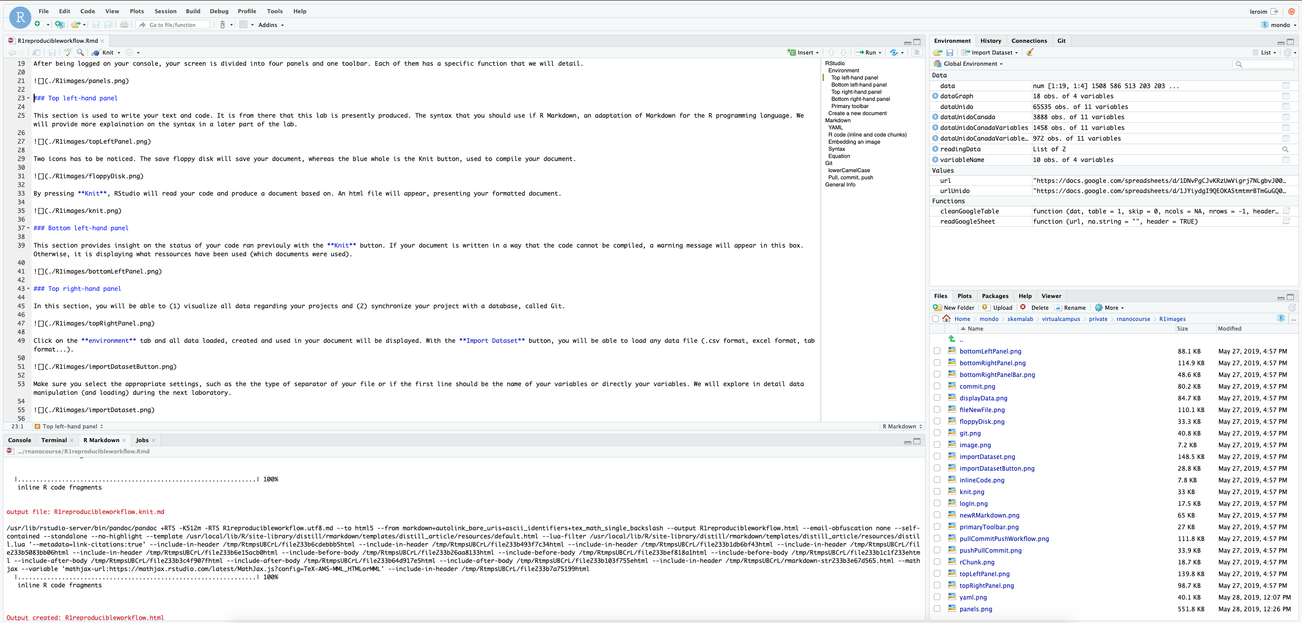
After being logged on your console, your screen is divided into four panels and one toolbar. Each of them has a specific function that we will detail.
Top left-hand panel
This section is used to write your text and code. It is from there that this first R nanocourse is presently produced. The syntax that you should use is R Markdown, an adaptation of Markdown for the R programming language. We will provide more explaination on the syntax in the next R nanocourses.
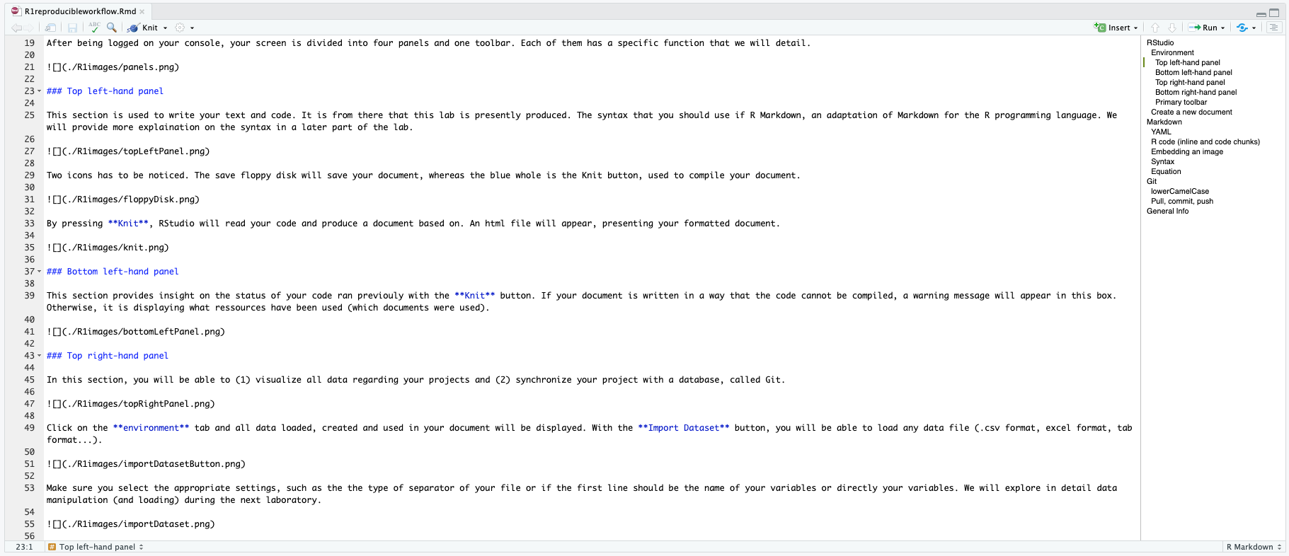
Two icons has to be noticed. The save floppy disk will save your document, whereas the blue whole is the Knit button, used to compile your document.

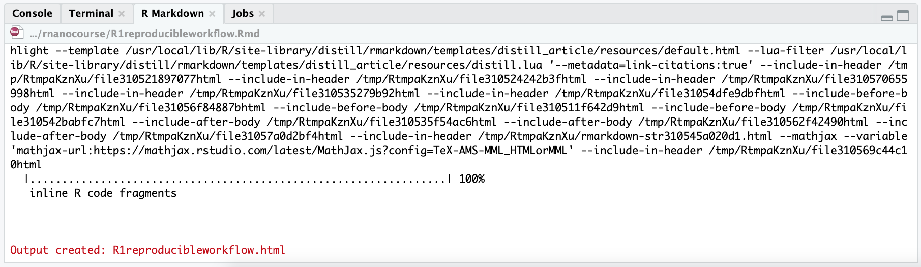
By pressing Knit, RStudio will read your code and produce a document. An html file will appear, presenting your formatted document.

By pressing the Document Outline icon, RStudio will show or hide the table of contents of your document.

Bottom left-hand panel
This section provides an insight on the status of your code ran previously with the Knit button. If your document is written in a way that the code cannot be compiled, a warning message will appear in this box. Otherwise, it will display the resources (documents) that have been used.
Top right-hand panel
In this section, you will be able to (1) visualize all data regarding your projects and (2) synchronize your project with a database, called Git.
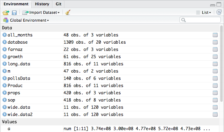
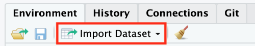
Click on the environment tab and all data loaded, created and used in your document will be displayed. With the Import Dataset button, you will be able to load any data file (.csv format, excel format, tab format…).
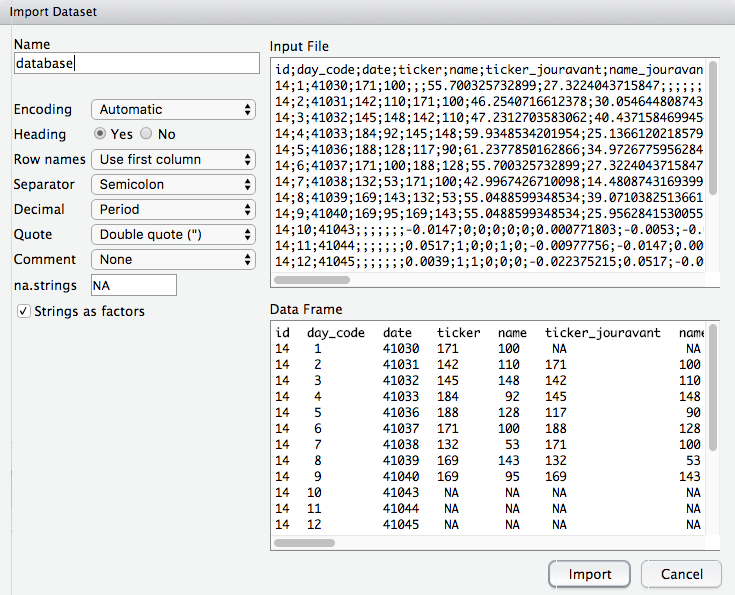
Make sure you select the appropriate settings, such as the the type of separator of your file or if the first line should be the name of your variables or directly your variables. We will explore in detail data manipulation (and loading) during the next R nanocourse.
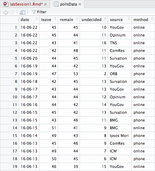
If you click on a specific data in the environment, the first 1000 lines of data will be displayed.
Click on the Git tab and you will see a list of files. We will describe in details how to properly use the Git in order to synchronize your project on an online database. This will be the last part of this lab.
Bottom right-hand panel
In the last panel, you will find all files available in your project under the Files tab. Note the path to reach each file, which may be useful when linking a picture or a dataset to the document your are editing. For example, the next picture will have a specific path, i.e.: ./R1images/bottomRightPanel.png. This indicates that the picture called bottomRightPanel.png is located in the pictures folder which in turn is in the labR1_files folder.
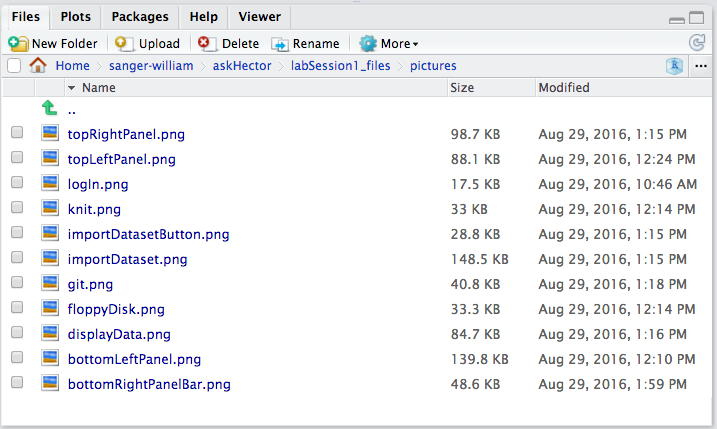
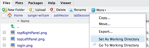
You can create a new folder by clicking on the New Folder button or change any setting of any file with the subsequent buttons. After clicking on the More button (blue engine), you will find the option to export any selected file. The option Set As Working Directory will indicate to RStudio from which file you are working from (in all the previous picture imports, the working directory was askHector, hence the ./ before each picture path details on how to use the Markdown syntax are provided in the next part).
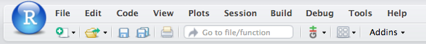
Primary toolbar
Several options are located in the primary upper toolbar. We will only explore how creating a new document in the following steps.
Create a new document
To create a new document, select File > New File > R Markdown.
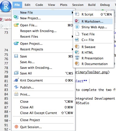
Select Document and enter the name of your new file with the default output format as HTML.
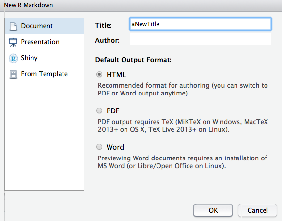
This will create a new file that you will be able to work with using the R Markdown syntax. Save your new file using the floppy disk icon seen previously.
At this point, you should be able to complete the two first achievements of the lab, namely:
- familiarize yourself with the RStudio Integrated Development Environment
- create your first document in RStudio
Markdown
Your newly created document will be written using the Markdown syntax. Such format incorporates R code (named chunks), provides the possibility to write mathematical equations in LaTeX and export your document to any format (presentation, html, .doc, PDF…).
YAML
At the beggining of the document lies the YAML, which dictates how the document will be formatted. The following lines of codes enables to write the author’s name, the date and the desired output (here an html document with a table of content).
---
title: "aNewTitle"
author: "John Doe"
date: "28/05/2019"
output: html_document
---
You can change the desired output by selecting a specific option:
- output: html_document -> html file
- output: pdf_document -> PDF
- output: word_document -> .docx document
- output: bearmer_presentation -> powerpoint-like presentation
- output: ioslides_presentation -> powerpoint-like presentation (html format)
- output: github_document -> format for GitHub
R code
Code Chunk
Reproducible research seeks to provide multiple analysis of a same dataset, and verify each result even thought data are changed during the process. Hence, by using R Markdown, it is possible to add R code, which are coding and programming parts to analyze data. In order to do so, you should write your R code in between 3 ticks called a R chunck, such as:
The first line will provide some descriptive statistics of a dataset (here named cars).
# provide some descriptive statistics
summary(cars)
## speed dist
## Min. : 4.0 Min. : 2.00
## 1st Qu.:12.0 1st Qu.: 26.00
## Median :15.0 Median : 36.00
## Mean :15.4 Mean : 42.98
## 3rd Qu.:19.0 3rd Qu.: 56.00
## Max. :25.0 Max. :120.00Whereas the second line of code will plot a graph of the previous data.
# plot a 2 axis graph
plot(cars)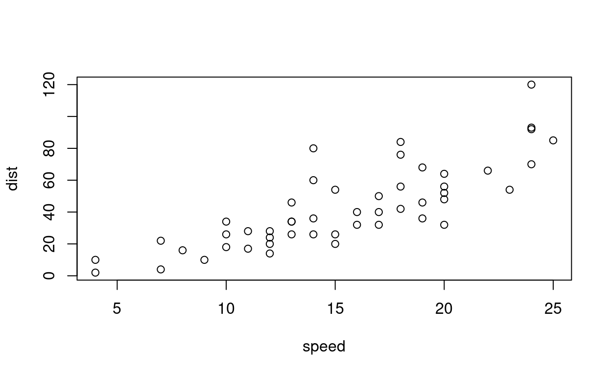
You should notice that a comment in a R chunck is written with a # before the beginning of the sentence.
Inline Code
For inline coding, instead of 3 ticks, a single tick with r is required, such as:
`r mean(cars$speed)`This code generate the average speed. Integrated in a sentence it looks like this:
The average speed of the dataset is equal to `r mean(cars$speed)` mile per hour.The result: The average speed of the dataset is equal to 15.4 mile per hour.
Embedding an image
Insert an image into your document by writting the following ponctuations: exclamation mark, brackets, parenthesis, with the path of the image inside parenthesis. For example:
Syntax
R Markdown has specific formatting settings that will be understood by RStudio.
- For bold text, encapsulate the text in between 2 stars. A bold text;
- For italic text, encapsulate the text in between 1 star. An italic text;
- For superscript text, encapsulate the text in between 1 circumflex.superscript;
- For linking a webpage to a text, provide the link with the following syntax: brackets parenthesis, with the link inside parenthesis and your text inside brackets. Link to the virtual campus.
A title has to be specified by a hash caracter (#). The number of # indicated the level of title: for example a second-order title will be preceeded by ##, whereas a third level title will be preceeded by ### (you have multiple examples in the present document).
Equation
Finally, you can write any equation using the LaTeX format in R Markdown. In order to do so, you have to insert your equation in a LaTeX format between two $.
For example, this equation:
$y_i= \alpha_0 + \alpha_1.x_1+\alpha_2.x_2+\alpha_3.x_3+\epsilon$Will generate this:
\(y_i= \alpha_0 + \alpha_1.x_1+\alpha_2.x_2+\alpha_3.x_3+\epsilon\)
By this point, you should be able to complete the third achievement of the lab, namely:
- understand the Markdown syntax and knit your document
Git
In this final section, we will present how to save your project in the RStudio console. Previously, we mentionned the blue floppy disk button located in the top left-hand panel. This button will only save your project locally, meaning that only you will be able to save and access the file. However, your project must be synchronized in an online server called Git (located in the top right-hand panel).
lowerCamelCase
All your files must be labelled in a specific syntax, called lowerCamelCase. No space/symbol/accent should be inside file names. For example, the name of a document should look like this: reproducibleNanocourse1.Rmd. The first word is in lower case whereas all subsequent words must be attached, with the first letter in capital.
Pull, commit, push
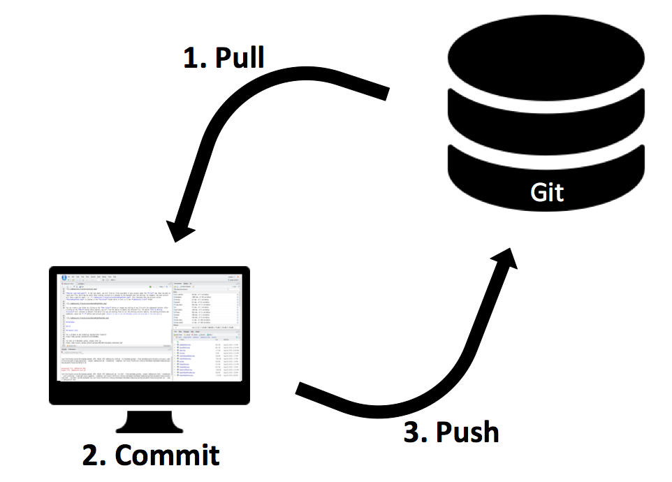
In order to synchronize your file with the instructors (which will be how every document for the semester will be saved and shared), three steps are required. First, select the Git tab in the top right-hand panel of the console.

- Pull means that you will import all files from the server which are not located in your local session;
- Commit means that you will make some changes to your files and that you want to mark them;
- Push means that you want to synchronize your local work with the server, hence add your contribution to the server.
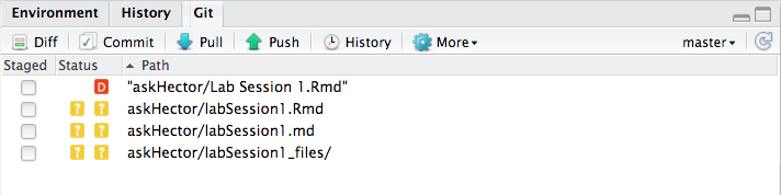
When you log in your console, always click on Pull in order to get the latest version of your files. When you have added some modifications to your project and that you want to save them, click on Commit. You will be redirected to the following panel:
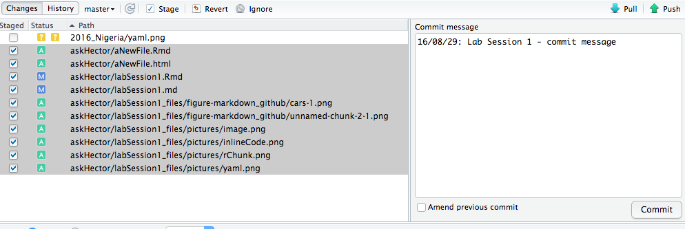
Select all files that you have created, deleted or modified and then click on the Stage button. You need to specify what kind of modification has been added in the commit message box. After clicking on Commit, your files will be marked. Now, click on Push in order to send all modifications to the server. That way, all your project will be synchronized online.
Remember: Pull > Commit > Push. This must become a reflex.
Now you should be able to successfully accomplish all four goals of this first R nanocourse.
References
For more on R Markdown syntax, please refer to: https://www.rstudio.com/wp-content/uploads/2015/02/rmarkdown-cheatsheet.pdf
Acknowledgments
To cite this course:
Warin, Thierry. 2020. “Nüance-R: R Nanocourses.” doi:10.6084/m9.figshare.11842416.v2.