Introduction

What makes R a compiling programming language is its facility to wrangle data on the fly. In this session, you will learn the basics of data manipulation. Based on the knowledge acquired in the previous sessions, you will transform complex datasets in order to represent and interpret results. We will use the United Nations Industrial Development Organization (UNIDO) dataset to illustrate this session.

Goals

At the end of the lecture, you should be able to:

1. know what a dataframe is;
2. add a column to an existing dataframe;
3. subset your dataframe based on a variable;
4. sort your dataframe;
5. transform your dataframe from long to wide form;
6. merge two datasets;
7. visualize your results.

You will go from a database of 655'350 points to a graphic made of 6 observations.

Keywords: data wrangling; RStudio; reproducible research

Nomenclature

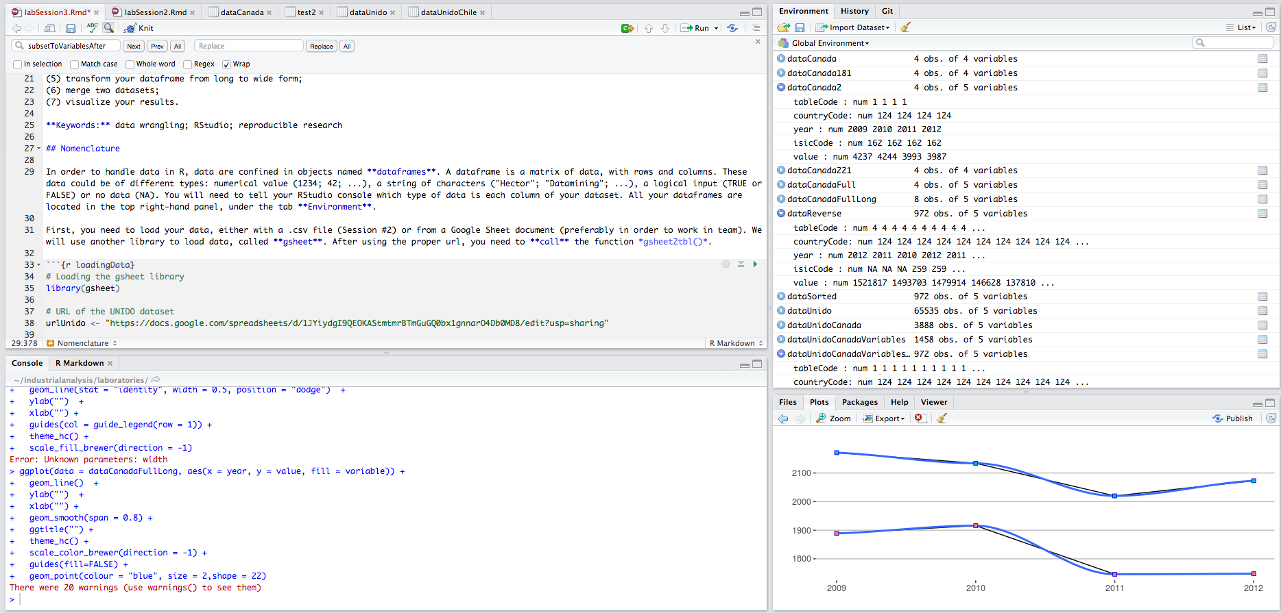
In order to handle data in R, data are confined in objects named dataframes. A dataframe is a matrix of data, with rows and columns. These data could be of different types: numerical value (1234; 42; ...), a string of characters ("Hector"; "Datamining"; ...), a logical input (TRUE or FALSE) or no data (NA). You will need to tell your RStudio console which type of data is each column of your dataset. All your dataframes are located in the top right-hand panel, under the tab Environment.

First, you need to load your data, either with a .csv file (R nanocourse #2) or from a Google Sheet document (preferably in order to work in team). For this nanocourse, we will use a Google Sheet document so, the package gsheet. After using the proper url, you need to call() the function gsheet2tbl().

We put the url in the gsheet2tbl() fuction.

# Loading the gsheet package
library(gsheet)

# Using the gsheet2tbl function to import the UNIDO dataset into the RStudio console
dataUnido <- gsheet2tbl("https://docs.google.com/spreadsheets/d/1uLaXke-KPN28-ESPPoihk8TiXVWp5xuNGHW7w7yqLCc/edit#gid=416085055")

# First 6 lines of the dataset
head(dataUnido)

Secondly, for each column, you need to assign a certain type of data. Here, you need to change the type of data of several columns to numerical values. For example, the column value is in character type.

To change the type of the column, you need to use the function as.numeric(). In order to manipulate a column, you must use a specific typology, with the symbol $: dataframe**$**column

# Transformation from character to numerical values
dataUnido$value <- as.numeric(dataUnido$value)
dataUnido$value <- as.numeric(dataUnido$value)
dataUnido$tableCode <- as.numeric(dataUnido$tableCode)
dataUnido$countryCode <- as.numeric(dataUnido$countryCode)
dataUnido$year <- as.numeric(dataUnido$year)
dataUnido$isicCode <- as.numeric(dataUnido$isicCode)

# Structure of the dataframe
summary(dataUnido)

##    tableCode      countryCode          year         isicCode   
##  Min.   : 1.00   Min.   : 31.00   Min.   :2005   Min.   : 106  
##  1st Qu.: 4.00   1st Qu.: 40.00   1st Qu.:2008   1st Qu.:1103  
##  Median : 5.00   Median : 76.00   Median :2010   Median :2219  
##  Mean   :11.14   Mean   : 98.24   Mean   :2009   Mean   :1955  
##  3rd Qu.:20.00   3rd Qu.:170.00   3rd Qu.:2011   3rd Qu.:2812  
##  Max.   :31.00   Max.   :203.00   Max.   :2012   Max.   :3320  
##  NA's   :1       NA's   :1        NA's   :1      NA's   :405   
##  isicCodeCombinaison     value            tableDefinitionCode
##  Length:65536        Min.   :-1.546e+09   Length:65536       
##  Class :character    1st Qu.: 1.030e+02   Class :character   
##  Mode  :character    Median : 1.950e+04   Mode  :character   
##                      Mean   : 2.164e+10                      
##                      3rd Qu.: 9.600e+07                      
##                      Max.   : 2.054e+14                      
##                      NA's   :23805                           
##   sourceCode         updateYear            unit          
##  Length:65536       Length:65536       Length:65536      
##  Class :character   Class :character   Class :character  
##  Mode  :character   Mode  :character   Mode  :character  
##                                                          
##                                                          
##                                                          
## 

If you want to change a column to a character type, you have to use the function as.character().

Add & delete a column

Now that you can work with your dataset, you may need to add another column to it. To do so, enter the name of your new column after the $ symbol and assign a value to it.

# Add a new column called 'newColumn'
dataUnido$newColumn <- 42

# Show the columns' name
colnames(dataUnido)

##  [1] "tableCode"           "countryCode"         "year"               
##  [4] "isicCode"            "isicCodeCombinaison" "value"              
##  [7] "tableDefinitionCode" "sourceCode"          "updateYear"         
## [10] "unit"                "newColumn"

# Show the column 'newColumn'
dataUnido[,"newColumn"]

You can manipulate this column, for example by multiplying it by 2 and adding 5 units.

# Multiply by 2 and add 5
dataUnido$newColumn <- dataUnido$newColumn * 2 + 5

# Show the column 'newColumn'
dataUnido[,"newColumn"]

In order to delete this column, you need to assign the value NULL to this new column.

# Delete the column named 'newColumn'
dataUnido$newColumn <- NULL

# Show columns' name
colnames(dataUnido)

##  [1] "tableCode"           "countryCode"         "year"               
##  [4] "isicCode"            "isicCodeCombinaison" "value"              
##  [7] "tableDefinitionCode" "sourceCode"          "updateYear"         
## [10] "unit"

Now, you know how to:

• load your dataframe,
• transform it,
• add or delete a particular column.

From this point, we will erase some variables in our dataset from UNIDO in order to simplify our manipulations.

# erasing non important variables
dataUnido$isicCodeCombinaison <- NULL
dataUnido$tableDefinitionCode <- NULL
dataUnido$sourceCode <- NULL
dataUnido$updateYear <- NULL
dataUnido$unit <- NULL

The resulting dataset is a dataframe of 65'535 lines and 5 columns.

# Provide first 6 lines of the dataframe
head(dataUnido)

# Provide the dimension of the dataframe
dim(dataUnido)

## [1] 65536     5

Subset of a dataset

The UNIDO dataset is extensive (10 columns and 65'535 rows). It gathers information (value) on several indicators (tableDefinitionCode) from countries (countryCode) over a period of time (2005 - 2012, year).

One may need to use only a subset of this dataset. For example, we would like to know the number of employees and the number of establishments of all sectors in Canada after 2008. Using the definition of the UNIDO dataset, this translates to:

1. Canada: dataUnido$countryCode == 124
2. number of employees OR (|) number of establishments: tableDefinitionCode == 04 | tableDefinitionCode == 01
   
3. after 2009: dataUnido$year > 2009

In order to create a subset of the initial dataset, you need to use the function filter() from the package dplyr.

# Loading the dplyr package
library(dplyr)

# Subset of dataUnido based on countryCode == Canada
dataUnidoCanada <- filter(dataUnido, countryCode == 124)

# First lines of the dataframe
head(dataUnidoCanada)

# Number of columns & rows
dim(dataUnidoCanada)

## [1] 3888    5

Now, our subset is composed of 3888 rows and 5 columns, all of them concerning Canada.

# Subset of dataUnidoCanada based on two variables (number of employees and establishments)
dataUnidoCanadaVariables <- filter(dataUnidoCanada, tableCode == 4 | tableCode == 1)

# First lines of the dataframe
head(dataUnidoCanadaVariables)

# Last lines of the dataframe
tail(dataUnidoCanadaVariables)

Our subset is now composed of 1458 rows and 5 columns, with the number of employees and establishments in Canada.

# Number of columns & rows
dim(dataUnidoCanadaVariables)

## [1] 1458    5

In order to select only observation after 2009, you need to reiterate the same manipulation, this time on the variable year.

# Subset of dataUnido based on countryCode == Canada
dataUnidoCanadaVariablesAfter2009 <- filter(dataUnidoCanadaVariables, year > 2009)

# First lines of the dataframe
head(dataUnidoCanadaVariablesAfter2009)

# Dimension of the dataframe
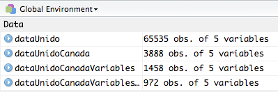
dim(dataUnidoCanadaVariablesAfter2009)

## [1] 972   5

The final dataset (dataUnidoCanadaVariablesAfter2009) is a dataframe of 972 rows and 5 columns. With the filter() function from the dplyr package, you can now manipule any dataset in order to filter and create a subset of it, based on any variable. In the following picture, you can see that each dataset is smaller and smaller than the previous one (these data are located in your environment panel).

To familiarize yourself with these manipulations, consider the following exercices:

Exercice 1: from the UNIDO database, create a dataframe concerning the number of employees in Canada; from 2009 to 2012

library(gsheet)
library(dplyr)
dataUnido <- gsheet2tbl("https://docs.google.com/spreadsheets/d/1uLaXke-KPN28-ESPPoihk8TiXVWp5xuNGHW7w7yqLCc/edit#gid=416085055")

dataUnido <- rename(dataUnido, Country=countryCode)
dataUnido <- rename(dataUnido, Year=year)
dataUnido <- rename(dataUnido, Employes=tableDefinitionCode)

dataUnido[,8:10]<-NULL
dataUnido$tableCode<-NULL
dataUnido$isicCode<-NULL
dataUnido$isicCodeCombinaison<-NULL

filter(dataUnido, Country==124 & Year==c(2009:2012) & Employes == 04)

Exercice 2: from the UNIDO database, create a dataframe concerning Dairy products from all country in 2011

library(gsheet)
library(dplyr)
dataUnido <- gsheet2tbl("https://docs.google.com/spreadsheets/d/1uLaXke-KPN28-ESPPoihk8TiXVWp5xuNGHW7w7yqLCc/edit#gid=416085055")

dataUnido <- rename(dataUnido, Country=countryCode)
dataUnido <- rename(dataUnido, Year=year)
dataUnido <- rename(dataUnido, Employes=tableDefinitionCode)

dataUnido[,8:10]<-NULL
dataUnido$tableCode<-NULL
dataUnido$isicCodeCombinaison<-NULL

dataUnidoFilter<-filter(dataUnido, isicCode==1520 & Year==2011 & Employes == 04)

dairyProducts<-arrange(dataUnidoFilter, desc(value))

dairyProducts

Sorting data

At the present moment, your dataframe is sort by alphabetical order. By using the arrange() function of the dplyr package, it is possible to sort your dataframe depending on a variable. This can be done in ascending order or in descending order.

# dataSorted will receive the dataframe dataUnidoCanadaVariablesAfter2009 sorted by the column value
dataSorted <- arrange(dataUnidoCanadaVariablesAfter2009, value)

# dataReverse is the opposite of dataSorted, i.e. the first lines will have the highest values
dataReverse <- arrange(dataUnidoCanadaVariablesAfter2009, desc(value))

We can compare both dataframes (dataSorted and dataReverse) to observe that they are arrange in different orders.

# first 6 lines of each dataset
head(dataSorted)

head(dataReverse)

Long and wide form

We can observe two types of layouts in a dataset:

• wide form: 1 column per variable (longitudinal data)
• long form: 1 column with all information (panel data)

# Loading reshape2
library(reshape2)

# Using dcast() to transform a long dataframe into a wide dataframe
wideData <- dcast(dataSorted, year + tableCode + countryCode ~ isicCode, value = value)

# First 6 lines
head(wideData)

# Dimension of the dataset
dim(wideData)

## [1]   6 165

# Loading reshape2
library(reshape2)

# Using melt() to transform from wide to long data
longData <- melt(wideData, id.vars=c("year", "tableCode", "countryCode"))

# Dimension of the dataframe
dim(longData)

## [1] 972   5

# First 6 lines
head(longData)

Merging datasets

The final step of this nanocourse is to merge several datasets together. Let's consider two datasets with the following settings:

First dataset, named dataCanada131, with:

• the number of employees: tableCode == 4
• in the textile sector: isicCode == 131
• from Canada: countryCode == 124
• after 2008: year > 2008

Second dataset, named dataCanada181, with:

• the number of employees: tableCode == 4
• in the printing sector: isicCode == 181
• from Canada: countryCode == 124
• after 2008: year > 2008

# Dataset for dataCanada
dataCanada131 <- filter(dataUnido, countryCode == 76)
dataCanada131 <- filter(dataCanada131, isicCode == 131)
dataCanada131 <- filter(dataCanada131, tableCode == 4)
dataCanada131 <- filter(dataCanada131, year > 2008)
dataCanada131 <- dcast(dataCanada131, year + tableCode + countryCode ~ isicCode, value = value)

head(dataCanada131)

# Dataset for dataCanada181
dataCanada181 <- filter(dataUnido, countryCode == 76)
dataCanada181 <- filter(dataCanada181, isicCode == 181)
dataCanada181 <- filter(dataCanada181, tableCode == 4)
dataCanada181 <- filter(dataCanada181, year > 2008)
dataCanada181 <- dcast(dataCanada181, year + tableCode + countryCode ~ isicCode, value = value)

head(dataCanada181)

In order to merge your datasets, you need to use the full_join() function from the dplyr package. The first 2 arguments are the name of the datasets, whereas the third argument is the named of the common columns (here year, tableCode and countryCode).

# Merging 2 datasets
dataCanadaFull <- full_join(dataCanada131, dataCanada181, c("year","tableCode","countryCode"))

# First 6 lines
head(dataCanadaFull)

Visualization

Finally, from the last dataset (dataCanadaFull), you can visualize your results by using the bar chart code seen in R nanocourse #2. First you transform your data into a long format, then you can use the bar chart code.

# Transform dataCanadaFull in long data format
dataCanadaFullLong <- melt(dataCanadaFull, id.vars=c("year", "tableCode", "countryCode"))

# Produce a bar chart
library(ggplot2)
library(ggthemes)
ggplot(data = dataCanadaFullLong, aes(x = year, y = value, fill = variable)) + 
  geom_bar(stat = "identity", width = 0.5, position = "dodge")  +  
  ylab("Number of employees")  +
  xlab("") +
  guides(col = guide_legend(row = 1)) +
  theme_hc() +
  scale_fill_brewer(direction = -1)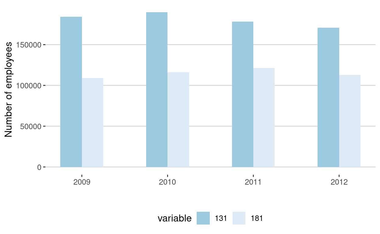

References

Acknowledgments

To cite this course: