The Structural Topic Model
This course demonstrates how to use the Structural Topic Model stm R package. The Structural Topic Model allows researchers to flexibly estimate a topic model that includes document-level metadata. Estimation is accomplished through a fast variational approximation. The stm package provides many useful features, including rich ways to explore topics, estimate uncertainty, and visualize quantities of interest.
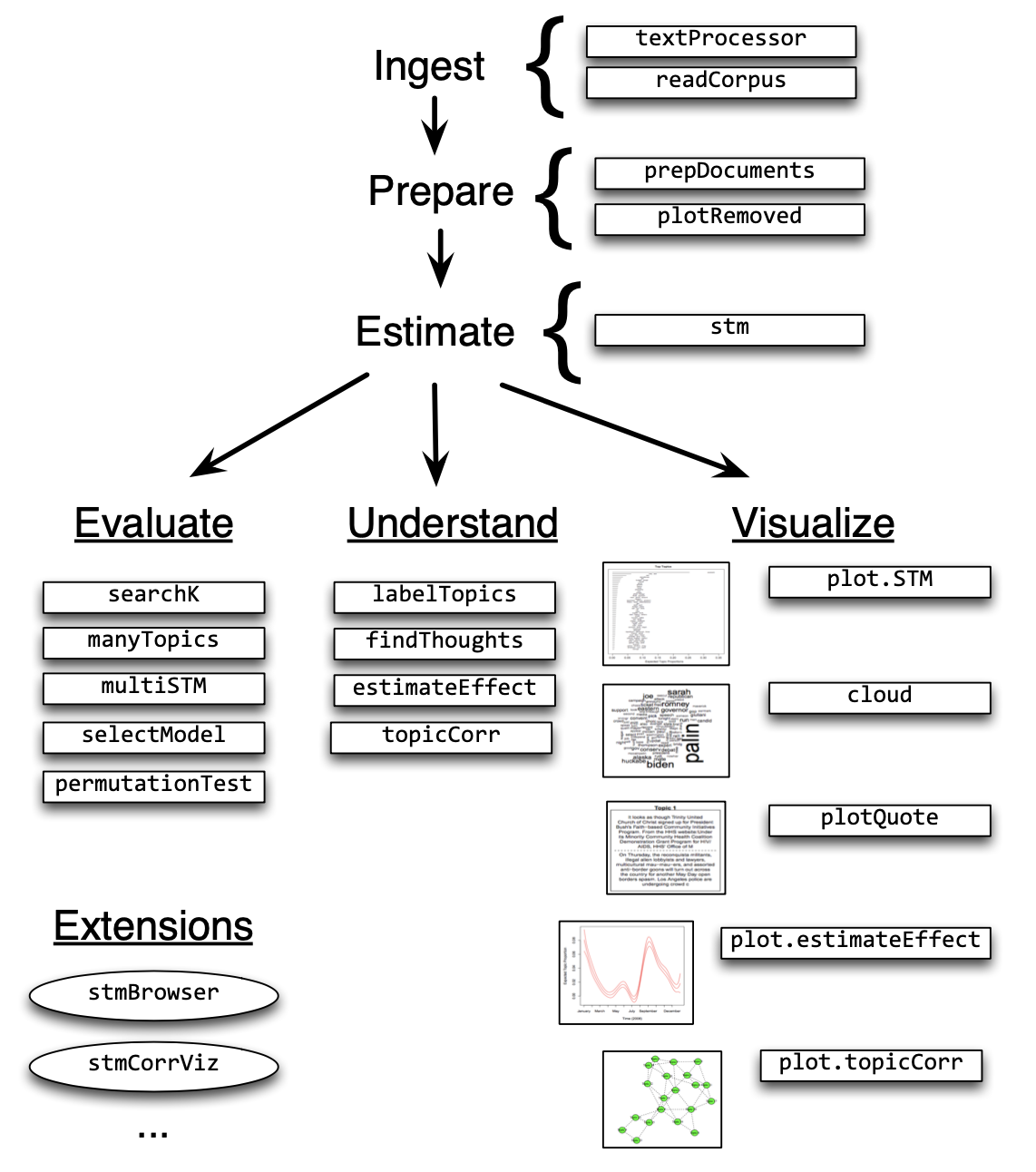
Figure 2: Heuristic description of selected stm package features
Ingest
Reading and processing text data
The first step is to load data into R. The stm package represents a text corpus in three parts:
- a documents list containing word indices and their associated counts,
- a vocab character vector containing the words associated with the word indices,
- a metadata matrix containing document covariates.
Reading in data from a “spreadsheet”:
The stm package provides a simple tool to quickly get started for a common use case:
- Get data: The researcher has stored text data alongside covariates related to the text in a spreadsheet, such as a .csv file that contains textual data and associated metadata.
- Read data: If the researcher reads this data into a R data frame,
- Convert and Process data: then the
stmpackage’s functiontextProcessorcan conveniently convert and processes the data to make it ready for analysis in thestmpackage.
Note: The model does not permit estimation when there are variables used in the model that have missing values. As such, it can be helpful to subset data to observations that do not have missing values for metadata that will be used in the stm model.
To illustrate how to use the stm package, a collection of blogposts about American politics that were written in 2008, from the CMU 2008 Political Blog Corpus (Eisenstein and Xing 2010) wil be used. The blogposts were gathered from six different blogs: American Thinker, Digby, Hot Air, Michelle Malkin, Think Progress, and Talking Points Memo. Each blog has its own particular political bent. The day within 2008 when each blog was written was also recorded. Thus for each blogpost, there is metadata available on the day it was written and the political ideology of the blog for which it was written. In this case, each blog post is a row in a .csv file, with the text contained in a variable called documents.
# Link spreadsheet:
# http://scholar.princeton.edu/sites/default/files/bstewart/files/poliblogs2008.csv

data <- read.csv("poliblogs2008.csv")
Pre-processing text content
It is often useful to engage in some processing of the text data before modeling it. The most common processing steps are stemming (reducing words to their root form), dropping punctuation and stop word removal (e.g., the, is, at). The textProcessor function implements each of these steps across multiple languages by using the stm package.
processed <- textProcessor(data$documents, metadata = data)
out <- prepDocuments(processed$documents, processed$vocab, processed$meta)
docs <- out$documents
vocab <- out$vocab
meta <- out$meta
Prepare
Associating text with metadata
After reading in the data, use the utility function prepDocuments to process the loaded data to make sure it is in the right format. prepDocuments also removes infrequent terms depending on the user-set parameter lower.thresh. The utility function plotRemoved will plot the number of words and documents removed for different thresholds.
For example, the user can use the following code to evaluate how many words and documents would be removed from the data set at each word threshold, which is the minimum number of documents a word needs to appear in order for the word to be kept within the vocabulary. Then the user can select their preferred threshold within prepDocuments.
Importantly, prepDocuments will also re-index all metadata/document relationships if any changes occur due to processing. If a document is completely removed due to pre-processing (for example because it contained only rare words), then prepDocuments will drop the corresponding row in the metadata as well. After reading in and processing the text data, it is important to inspect features of the documents and the associated vocabulary list to make sure they have been correctly pre-processed.
plotRemoved(processed$documents, lower.thresh = seq(1, 200, by = 100))
out <- prepDocuments(processed$documents, processed$vocab, processed$meta, lower.thresh = 15)
From here, researchers are ready to estimate a structural topic model.
Estimate
Estimating the structural topic model
The data import process will output documents, vocabulary and metadata that can be used for an analysis. In this section, let's see how to estimate the STM. Next we move to a range of functions to evaluate, understand, and visualize the fitted model object.
The key innovation of the STM is that it incorporates metadata into the topic modeling framework. In STM, metadata can be entered in the topic model in two ways:
- topical prevalence: Metadata covariates for topical prevalence allow the observed metadata to affect the frequency with which a topic is discussed.
- topical content: Covariates in topical content allow the observed metadata to affect the word rate use within a given topic – that is, how a particular topic is discussed.
Estimation for both topical prevalence and content proceeds via the workhorse stm function.
Estimation with topical prevalence parameter
In this example, let's use the ratings variable (blog ideology) as a covariate in the topic prevalence portion of the model with the CMU Poliblog data described above. Each document is modeled as a mixture of multiple topics.
Topical prevalence captures how much each topic contributes to a document. Because different documents come from different sources, it is natural to want to allow this prevalence to vary with metadata that we have about document sources.
We will let prevalence be a function of the “rating” variable, which is coded as either “Liberal” or “Conservative,” and the variable “day” which is an integer measure of days running from the first to the last day of 2008. To illustrate, let's estimate a 20 topic STM model. The user can then pass the output from the model, poliblogPrevFit, through the various functions discussed below (e.g., the plot method for ‘STM’ objects) to inspect the results.
If a user wishes to specify additional prevalence covariates, she would do so using the standard formula notation in R. A feature of the stm function is that “prevalence” can be expressed as a formula that can include multiple covariates and factorial or continuous covariates. For example, by using the formula setup you can enter other covariates additively. Additionally users can include more flexible functional forms of continuous covariates, including standard transforms like log(), as well as ns() or bs() from the splines package.
The stm package also includes a convenience function s(), which selects a fairly flexible b-spline basis. In the current example, the variable day is allowed to be estimated with a spline. Interactions between covariates can also be added using the standard notation for R formulas.
In the example below, we enter in the variables additively, by allowing for the day variable, an integer variable measuring which day the blog was posted, to have a non-linear relationship in the topic estimation stage.
poliblogPrevFit <- stm(documents = out$documents, vocab = out$vocab, K = 20, prevalence = ~rating + s(day), max.em.its = 75, data = out$meta, init.type = "Spectral")The model is set to run for a maximum of 75 EM iterations (controlled by max.em.its). Convergence is monitored by the change in the approximate variational lower bound. Once the bound has a small enough change between iterations, the model is considered converged.
Evaluate
Model selection and search
Model initialization for a fixed number of topics
As with all mixed-membership topic models, the posterior is intractable and non-convex, which creates a multi-modal estimation problem that can be sensitive to initialization. Put differently, the answers the estimation procedure comes up with may depend on starting values of the parameters (e.g., the distribution over words for a particular topic).
There are two approaches to dealing with this that the stm package facilitates.
The first is to use an initialization based on the method of moments, which is deterministic and globally consistent under reasonable conditions (Arora et al. 2013; Roberts et al. 2016a). This is known as a spectral initialization because it uses a spectral decomposition (non-negative matrix factorization) of the word co-occurrence matrix. In practice, this initialization is very helpful. This can be chosen by setting
init.type = "Spectral"in thestmfunction. This option is used in the above example. This means that no matter the seed that is set, the same results will be generated. When the vocabulary is larger than 10,000 words, the function will temporarily subset the vocabulary size for the duration of the initialization.The second approach is to initialize the model with a short run of a collapsed Gibbs sampler for LDA. For completeness researchers can also initialize the model randomly, but this is generally not recommended. In practice, the spectral initialization is generally recommended as it has been found that it to produce the best results consistently (Roberts et al. 2016a).
Model selection for a fixed number of topics
When not using the spectral initialization, the analyst should estimate many models, each from different initializations, and then evaluate each model according to some separate standard (several are provided below).
The function selectModel automates this process to facilitate finding a model with desirable properties. Users specify the number of “runs,” which in the example below is set to 20. selectModel first casts a net where “run” (below 10) models are run for two EM steps, and then models with low likelihoods are discarded.
Next, the default returns the 20% of models with the highest likelihoods, which are then run until convergence or the EM iteration maximum is reached. Notice that options for the stm function can be passed to selectModel, such as max.em.its. If users would like to select a larger number of models to be run completely, this can also be set with an option specified in the help file for this function.
poliblogSelect <- selectModel(out$documents, out$vocab, K = 20, prevalence = ~rating + s(day), max.em.its = 75, data = out$meta, runs = 20, seed = 8458159)In order to select a model for further investigation, users must choose one of the candidate models’ outputs from selectModel. To do this, plotModels can be used to plot two scores: semantic coherence and exclusivity for each model and topic. Each of these criteria are calculated for each topic within a model run.
The plotModels function calculates the average across all topics for each run of the model and plots these by labeling the model run with a numeral. Often users will select a model with desirable properties in both dimensions (i.e., models with average scores towards the upper right side of the plot).
plotModels(poliblogSelect, pch = c(1, 2, 3, 4), legend.position = "bottomright")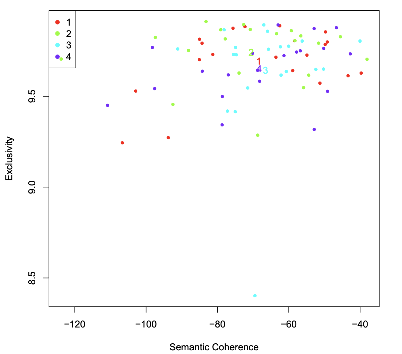
Figure 3: Plot of selectModel results. Numerals represent the average for each model, and dots represent topic specific scores
As shown in Figure 3, the plotModels function also plots each topic’s values, which helps give a sense of the variation in these parameters. For a given model, the user can plot the semantic coherence and exclusivity scores with the topicQuality function.
Next the user would want to select one of these models to work with. For example, the third model could be extracted from the object that is outputted by selectModel.
selectedmodel <- poliblogSelect$runout[[3]]Model search across numbers of topics
STM assumes a fixed user-specified number of topics. There is not a “right” answer to the number of topics that are appropriate for a given corpus (Grimmer and Stewart 2013), but the function searchK uses a data-driven approach to selecting the number of topics. The function will perform several automated tests to help choose the number of topics including calculating the held-out log-likelihood (Wallach, Murray, Salakhutdinov, and Mimno 2009) and performing a residual analysis (Taddy 2012).
For example, one could estimate a STM model for 7 and 10 topics and compare the results along each of the criteria. The default initialization is the spectral initialization due to its stability.
This function will also calculate a range of quantities of interest, including the average exclusivity and semantic coherence.
storage <- searchK(out$documents, out$vocab, K = c(7, 10), prevalence = ~rating + s(day), data = meta)There is another more preliminary selection strategy based on work by Lee and Mimno (2014). When initialization type is set to "Spectral" the user can specify \(K = 0\) to use the algorithm of Lee and Mimno (2014) to select the number of topics. The core idea of the spectral initialization is to approximately find the vertices of the convex hull of the word co-occurrences.
The algorithm of Lee and Mimno (2014) projects the matrix into a low dimensional space using t-distributed stochastic neighbor embedding (Van der Maaten 2014) and then exactly solves for the convex hull. This has the advantage of automatically selecting the number of topics. The added randomness from the projection means that the algorithm is not deterministic like the standard "Spectral" initialization type. Running it with a different seed can result in not only different results but a different number of topics. This procedure has no particular statistical guarantees and should not be seen as estimating the “true” number of topics. However it can be useful to start and has the computational advantage that it only needs to be run once.
Understand
Interpreting the STM by plotting and inspecting results
After choosing a model, the user must next interpret the model results. There are many ways to investigate the output, such as inspecting the words associated with topics or the relationship between metadata and topics. To investigate the output of the model, the stm package provides a number of options.
- Displaying words associated with topics (labelTopics, plot method for ‘STM’ objects with argument
type = "labels", sageLabels, plot method for ‘STM’ objects with argumenttype = "perspectives") or documents highly associated with particular topics (findThoughts, plotQuote). - Estimating relationships between metadata and topics as well as topical content (estimateEffect).
- Calculating topic correlations (topicCorr)
Understanding topics through words and example documents
Two approaches are describe for users to explore the topics that have been estimated. The first approach is to look at collections of words that are associated with topics. The second approach is to examine actual documents that are estimated to be highly associated with each topic. Both of these approaches should be used. Below, the 20 topic model estimated with the spectral initialization is used.
To explore the words associated with each topic, the labelTopics function can be used. For models where a content covariate is included sageLabels can also be used. Both these functions will print words associated with each topic to the console. The function by default prints several different types of word profiles, including highest probability words and FREX words.
FREX weights words by their overall frequency and how exclusive they are to the topic (calculated as given in Equation 6).13 Lift weights words by dividing by their frequency in other topics, therefore giving higher weight to words that appear less frequently in other topics. For more information on lift, see Taddy (2013).
Similar to lift, score divides the log frequency of the word in the topic by the log frequency of the word in other topics. For more information on score, see the lda R package. In order to translate these results to a format that can easily be used within a paper, the plot method for ‘STM’ objects with argument type = "labels" will print topic words to a graphic device. Notice that in this case, the labels option is specified as the plot method for ‘STM’ objects has several functionalities that is described below (the options for "perspectives" and "summary").
labelTopics(poliblogPrevFit, c(6, 13, 18))To examine documents that are highly associated with topics the findThoughts function can be used. This function will print the documents highly associated with each topic.
Reading these documents is helpful for understanding the content of a topic and interpreting its meaning. Using syntax from data.table (Dowle and Srinivasan 2017) the user can also use findThoughts to make complex queries from the documents on the basis of topic proportions.
In our example, for expositional purposes, the length of the document is restricted to the first 200 characters. We see that Topic 6 describes discussions of the Obama and McCain campaigns during the 2008 presidential election. Topic 18 discusses the Bush administration.
To print example documents to a graphics device, plotQuote can be used. The results are displayed in Figure 4.
thoughts6 <- findThoughts(poliblogPrevFit, texts = shortdoc, n = 2, topics = 6)$docs[[1]]
thoughts18 <- findThoughts(poliblogPrevFit, texts = shortdoc, n = 2, topics = 18)$docs[[1]]
par(mfrow = c(1, 2), mar = c(0.5, 0.5, 1, 0.5))
plotQuote(thoughts6, width = 30, main = "Topic 6")
plotQuote(thoughts18, width = 30, main = "Topic 18")
Figure 4: Example documents highly associated with Topics 6 and 18
Estimating metadata/topic relationships
Estimating the relationship between metadata and topics is a core feature of the stm package. These relationships can also play a key role in validating the topic model’s usefulness (Grimmer 2010; Grimmer and Stewart 2013). While stm estimates the relationship for the (K − 1) simplex, the workhorse function for extracting the relationships and associated uncertainty on all K topics is estimateEffect. This function simulates a set of parameters which can then be plotted.
Typically, users will pass the same model of topical prevalence used in estimating the STM to the estimateEffect function. The syntax of the estimateEffect function is designed so users specify the set of topics they wish to use for estimation, and then a formula for metadata of interest. Different estimation strategies and standard plot design features can be used by calling the plot method for ‘estimateEffect’ objects.
estimateEffect can calculate uncertainty in several ways. The default is "Global", which will incorporate estimation uncertainty of the topic proportions into the uncertainty estimates using the method of composition. If users do not propagate the full amount of uncertainty, e.g., in order to speed up computational time, they can choose uncertainty = "None", which will generally result in narrower confidence intervals because it will not include the additional estimation uncertainty. Calling summary on the ‘estimateEffect’ object will generate a regression table.
out$meta$rating <- as.factor(out$meta$rating)
prep <- estimateEffect(1:20 ~ rating + s(day), poliblogPrevFit, meta = out$meta, uncertainty = "Global")
summary(prep, topics = 1)
Visualize
Presenting STM results
The functions described previously to understand STM results can be leveraged to visualize results for formal presentation. In this section let's focus on several of these visualization tools.
Summary visualization
Corpus level visualization can be done in several different ways. The first relates to the expected proportion of the corpus that belongs to each topic. This can be plotted using the plot method for ‘STM’ objects with argument type = "summary". An example from the political blogs data is given in Figure 5. We see, for example, that the Sarah Palin/vice president Topic 13 is actually a relatively minor proportion of the discourse. The most common topic is a general topic full of words that bloggers commonly use, and therefore is not very interpretable. The words listed in the figure are the top three words associated with the topic.
plot(poliblogPrevFit, type = "summary", xlim = c(0, 0.3))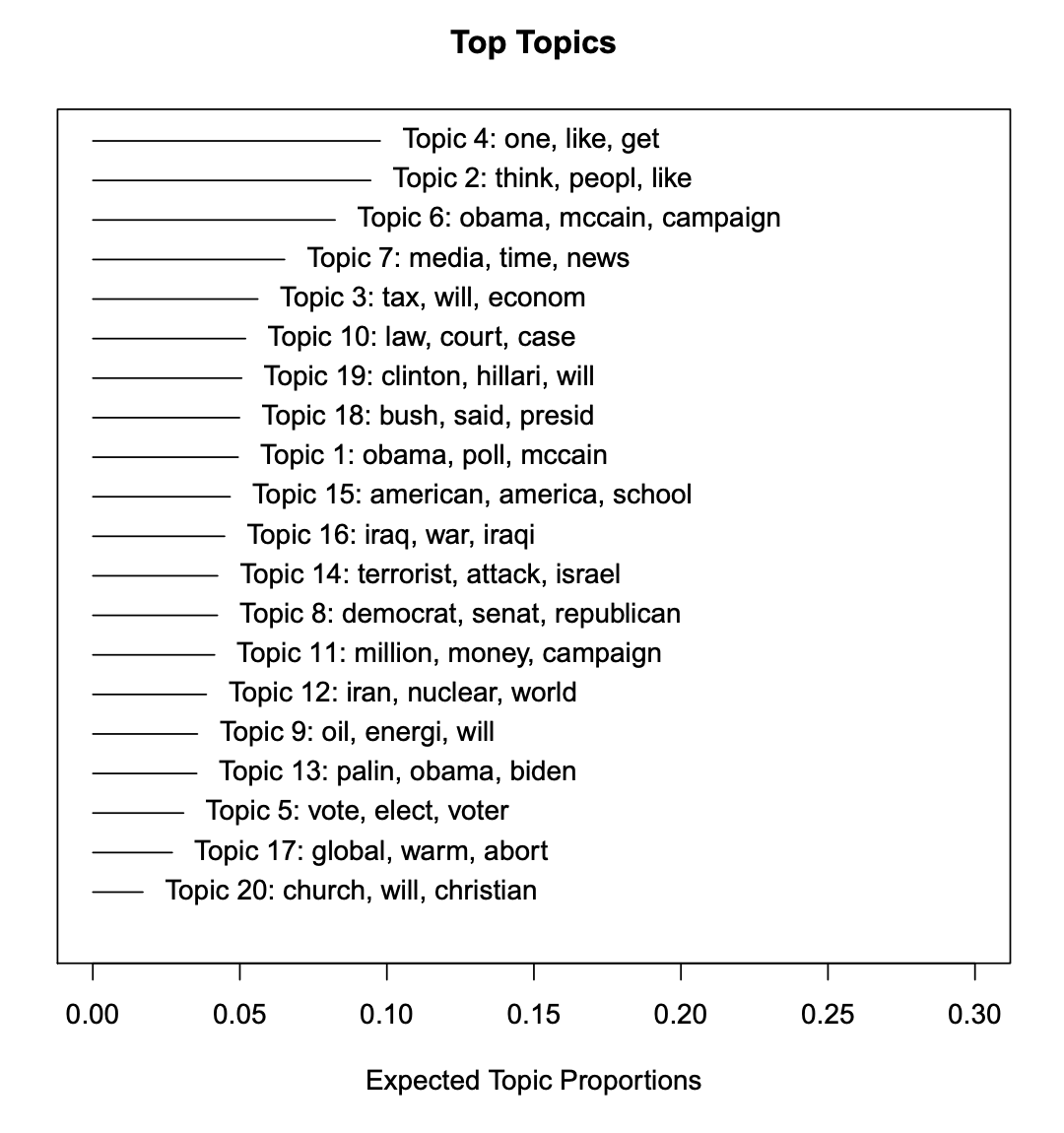
Figure 5: Graphical display of topical prevalence contrast
In order to plot features of topics in greater detail, there are a number of options in the plot method for ‘STM’ objects, such as plotting larger sets of words highly associated with a topic or words that are exclusive to the topic. Furthermore, the cloud function will plot a standard word cloud of words in a topic16 and the plotQuote function provides an easy to use graphical wrapper such that complete examples of specific documents can easily be included in the presentation of results.
Metadata/topic relationship visualization
Now let's discuss plotting metadata/topic relationships, as the ability to estimate these relationships is a core advantage of the STM model. The core plotting function is the plot method for ‘estimateEffect’ objects, which handles the output of estimateEffect.
First, users must specify the variable that they wish to use for calculating an effect. If there are multiple variables specified in estimateEffect, then all other variables are held at their sample median. These parameters include the expected proportion of a document that belongs to a topic as a function of a covariate, or a first difference type estimate, where topic prevalence for a particular topic is contrasted for two groups (e.g., liberal versus conservative). estimateEffect should be run and the output saved before plotting when it is time intensive to calculate uncertainty estimates and/or because users might wish to plot different quantities of interest using the same simulated parameters from estimateEffect. The output can then be plotted.
When the covariate of interest is binary, or users are interested in a particular contrast, the method = "difference" option will plot the change in topic proportion shifting from one specific value to another. Figure 6 gives an example. For factor variables, users may wish to plot the marginal topic proportion for each of the levels ("pointestimate").
plot(prep, covariate = "rating", topics = c(6, 13, 18), model = poliblogPrevFit, method = "difference", cov.value1 = "Liberal", cov.value2 = "Conservative", xlab = "More Conservative ... More Liberal", main = "Effect of Liberal vs. Conservative", xlim = c(-0.1, 0.1), labeltype = "custom", custom.labels = c("Obama/McCain", "Sarah Palin", "Bush Presidency"))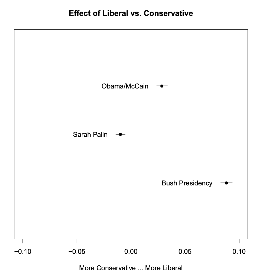
Figure 6: Graphical display of topical prevalence contrast
We see Topic 6 is strongly used slightly more by liberals as compared to conservatives, while Topic 13 is close to the middle but still conservative-leaning. Topic 18, the discussion of Bush, was largely associated with liberal writers, which is in line with the observed trend of conservatives distancing from Bush after his presidency.
Notice how the function makes use of standard labeling options available in the native plot() function. This allows the user to customize labels and other features of their plots. Note that in the package, generics are leverage for the plot functions. As such, one can simply use plot and rely on method dispatch.
When users have variables that they want to treat continuously, users can choose between assuming a linear fit or using splines. In the previous example, the day variable is allowed to have a non-linear relationship in the topic estimation stage. Then plot its effect on topics. In Figure 7, the relationship between time and the vice president topic, Topic 13, is plotted. The topic peaks when Sarah Palin became John McCain’s running mate at the end of August in 2008.
plot(prep, "day", method = "continuous", topics = 13, model = z, printlegend = FALSE, xaxt = "n", xlab = "Time (2008)")
monthseq <- seq(from = as.Date("2008-01-01"), to = as.Date("2008-12-01"), by = "month")
monthnames <- months(monthseq)
axis(1,at = as.numeric(monthseq) - min(as.numeric(monthseq)), labels = monthnames)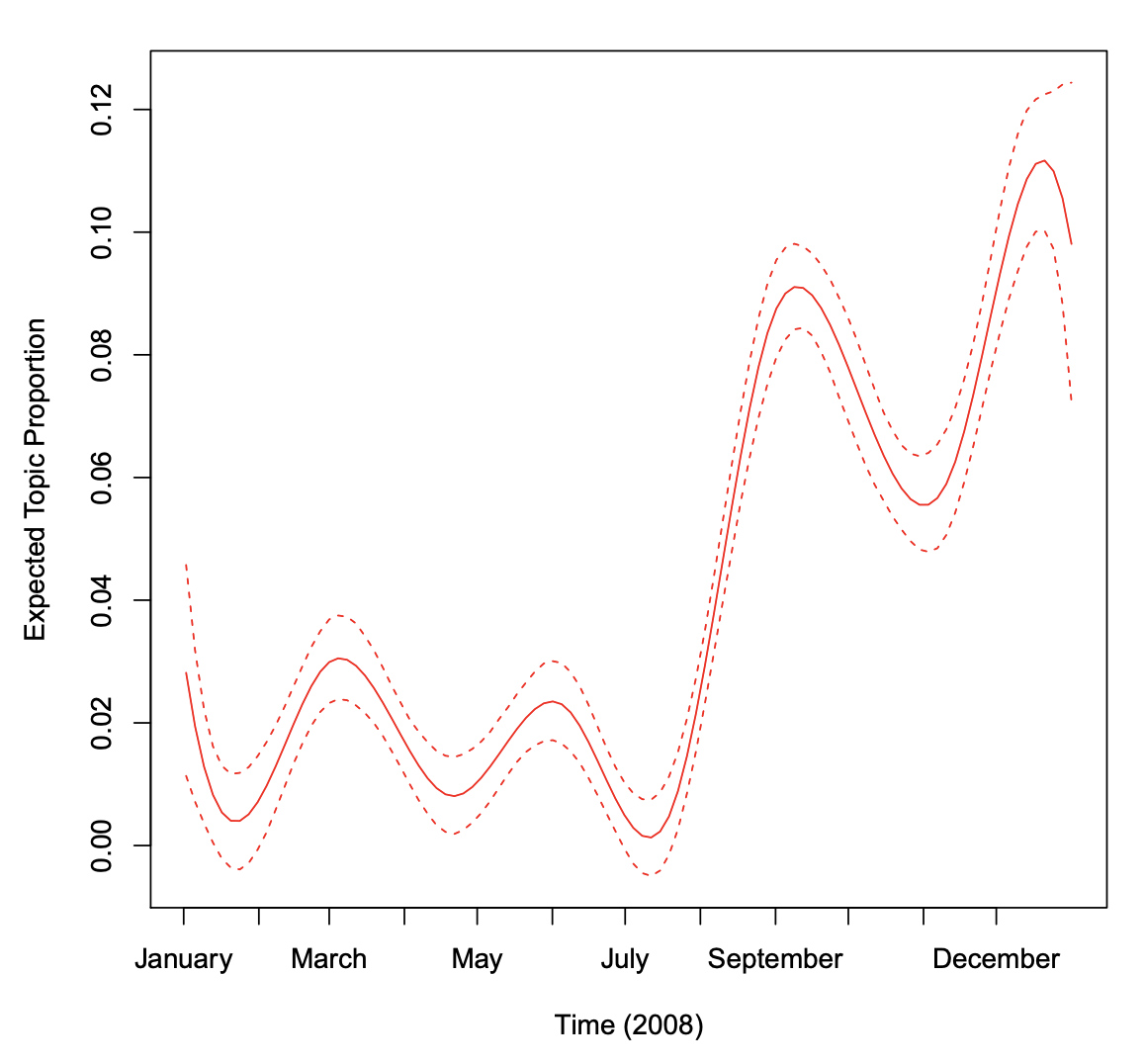
Figure 7: Graphical display of topic prevalence. Topic 13 prevalence is plotted as a smooth function of day, holding rating at sample median, with 95% confidence intervals.
Topical content
Let's also plot the influence of a topical content covariate. A topical content variable allows for the vocabulary used to talk about a particular topic to vary. First, the STM must be fit with a variable specified in the content option. In the below example, the variable rating serves this purpose. It is important to note that this is a completely new model, and so the actual topics may differ in both content and numbering compared to the previous example where no content covariate was used.
poliblogContent <- stm(out$documents, out$vocab, K = 20, prevalence =~ rating + s(day), content =~ rating, max.em.its = 75, data = out$meta, init.type = "Spectral")Next, the results can be plotted using the plot method for ‘STM objects with argument type = "perspectives". This function shows which words within a topic are more associated with one covariate value versus another.
plot(poliblogContent, type = "perspectives", topics = 10)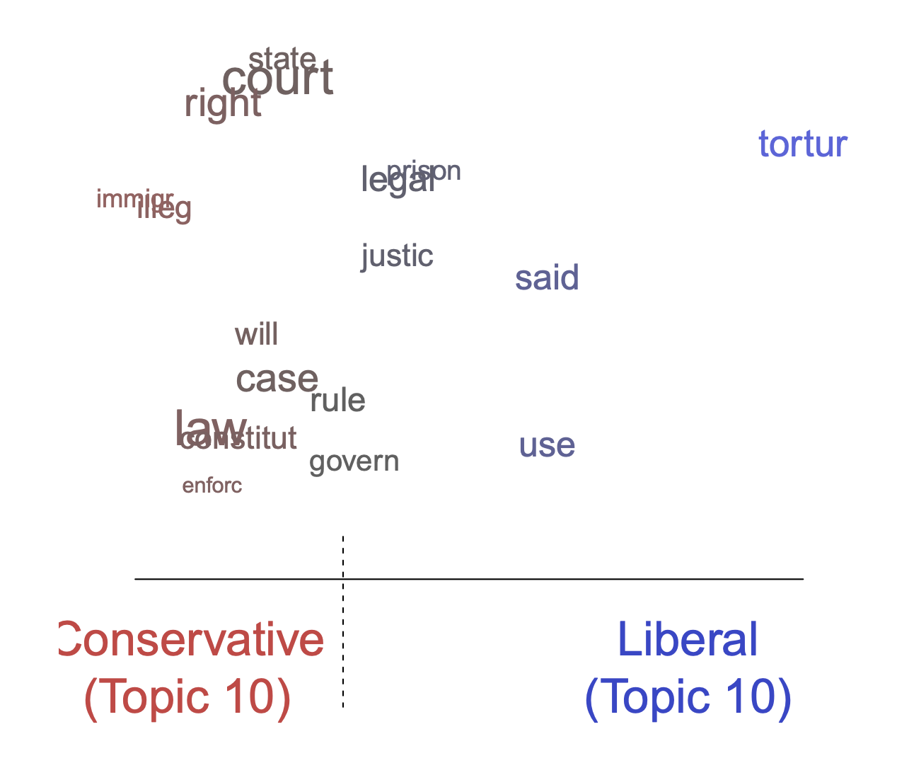
Figure 8: Graphical display of topical perspectives.
In Figure 8, vocabulary differences by rating is plotted for Topic 10. Topic 10 is related to Guantanamo. Its top FREX words were “detaine, prison, court, illeg, tortur, enforc, guantanamo”. However, Figure 8 indicates how liberals and conservatives talk about this topic differently. In particular, liberals emphasized “torture” whereas conservatives emphasized typical court language such as “illegal” and “law.”
This function can also be used to plot the contrast in words across two topics. To show this, let's go back to the original model that did not include a content covariate and let's contrast Topic 16 (Iraq war) and 18 (Bush presidency). The results are plotted in Figure 9.
plot(poliblogPrevFit, type = "perspectives", topics = c(16, 18))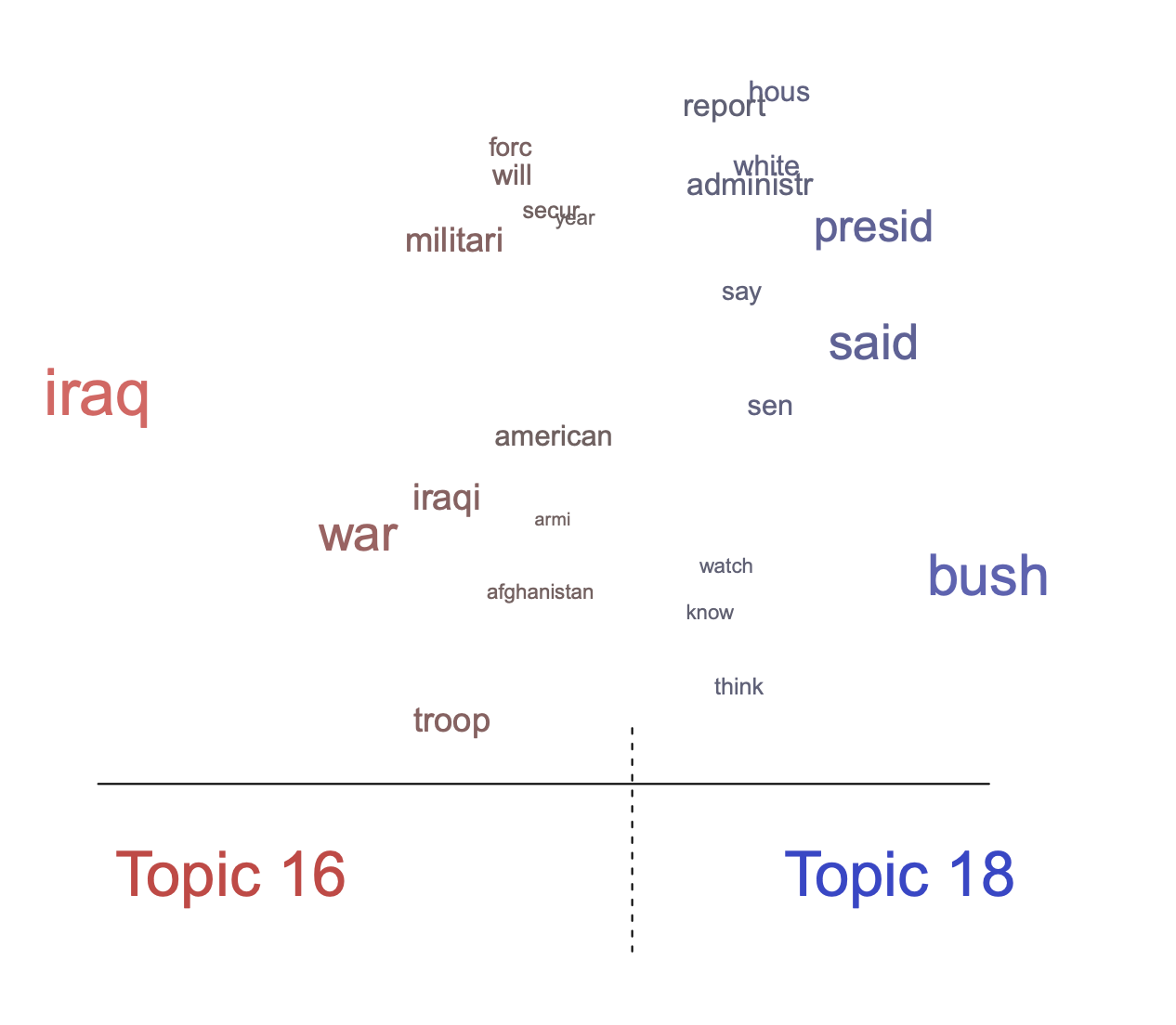
Figure 9: Graphical display of topical contrast between Topics 16 and 18.
Plotting covariate interactions
Another modification that is possible in this framework is to allow for interactions between covariates such that one variable may “moderate” the effect of another variable. In this example, the STM is re-estimated to allow for an interaction between day (entered linearly) and rating. Then in estimateEffect() the same interaction is included. This allows us in the plot method for ‘estimateEffect’ objects to have this interaction plotted. The results are displayed in Figure 10 for Topic 20 (Bush administration). You can observe that conservatives never wrote much about this topic, whereas liberals discussed this topic a great deal, but over time the topic diminished in salience.
poliblogInteraction <- stm(out$documents, out$vocab, K = 20, prevalence =~ rating * day, max.em.its = 75, data = out$meta, init.type = "Spectral")The day variable is entered here linearly for simplicity; however, you can use the software to estimate interactions with non-linear variables such as splines. However, the plot method for ‘estimateEffect’ objects only supports interactions with at least one binary effect modification covariate.
prep <- estimateEffect(c(16) ~ rating * day, poliblogInteraction, + metadata = out$meta, uncertainty = "None")
plot(prep, covariate = "day", model = poliblogInteraction, + method = "continuous", xlab = "Days", moderator = "rating", moderator.value = "Liberal", linecol = "blue", ylim = c(0, 0.12), printlegend = FALSE)

plot(prep, covariate = "day", model = poliblogInteraction, method = "continuous", xlab = "Days", moderator = "rating", moderator.value = "Conservative", linecol = "red", add = TRUE, printlegend = FALSE)

legend(0, 0.06, c("Liberal", "Conservative"), lwd = 2, col = c("blue", "red"))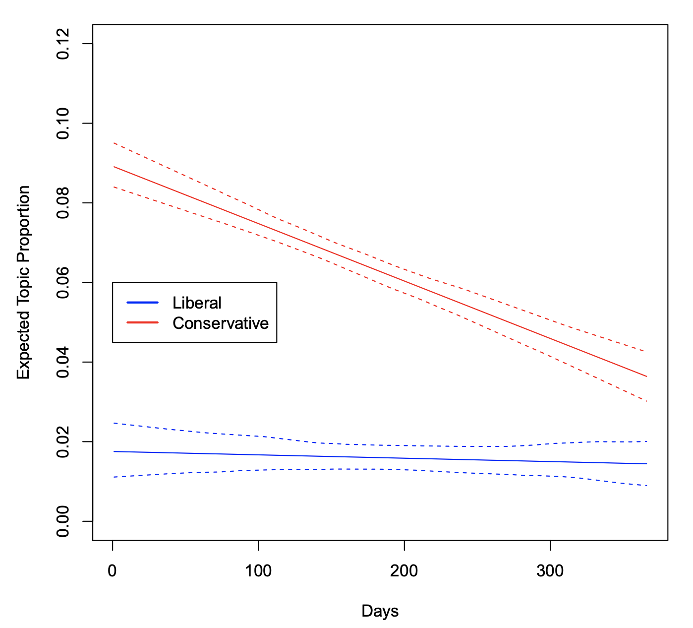
Figure 10: Graphical display of topical content. This plots the interaction between time (day of blog post) and rating (liberal versus conservative). Topic 16 prevalence is plotted as linear function of time, holding the rating at either 0 (Liberal) or 1 (Conservative). Were other variables included in the model, they would be held at their sample medians.
Extend: Additional tools for interpretation and visualization
There are multiple other ways to visualize results from a STM model. Topics themselves may be nicely presented as a word cloud. For example, Figure 11 uses the cloud function to plot a word cloud of the words most likely to occur in blog posts related to the vice president topic in the 2008 election.
cloud(poliblogPrevFit, topic = 13, scale = c(2, 0.25))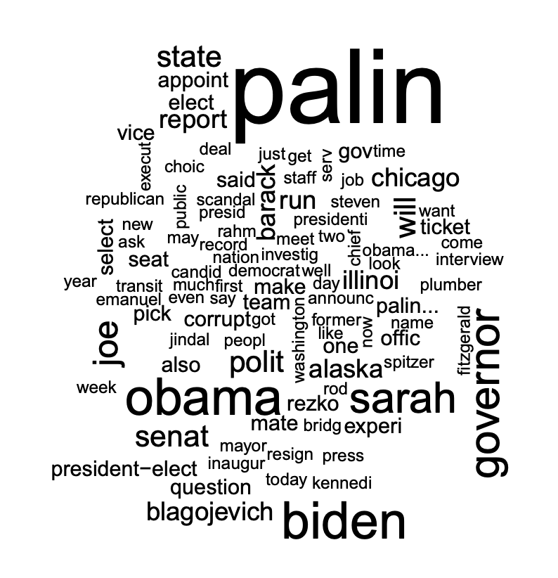
Figure 11: Word cloud display of vice president topic
In addition, the structural topic model permits correlations between topics. Positive correlations between topics indicate that both topics are likely to be discussed within a document.
These can be visualized using the plot method for ‘topicCorr’ objects. The user can specify a correlation threshold. If two topics are correlated above that threshold, then those two topics are considered to be linked. After calculating which topics are correlated with one another, the plot method for ‘topicCorr’ objects produces a layout of topic correlations using a force-directed layout algorithm, which it's presented in Figure 12. The correlation graph can be used to observe the connection between Topics 12 (Iraq War) and 20 (Bush administration). The plot method for ‘topicCorr’ objects has several options that are described in the help file.
mod.out.corr <- topicCorr(poliblogPrevFit)
plot(mod.out.corr)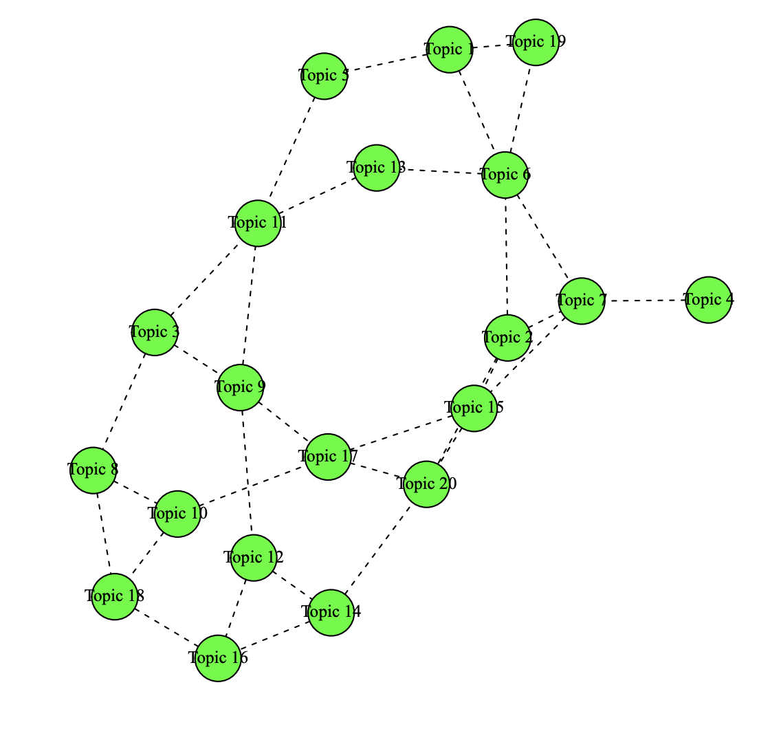
Figure 12: Graphical display of topic correlations.
Finally, there are several add-on packages that take output from a structural topic model and produce additional visualizations. In particular, the stmBrowser package (Freeman, Chuang, Roberts, Stewart, and Tingley 2015) contains functions to write out the results of a structural topic model to a d3 based web browser. The browser facilitates comparing topics, analyzing relationships between metadata and topics, and reading example documents.
The stmCorrViz package (Coppola, Roberts, Stewart, and Tingley 2016) provides a different d3 visualization environment that focuses on visualizing topic correlations using a hierarchical clustering approach that groups topics together. The function toLDAvis enables export to the LDAvis package (Sievert and Shirley 2015) which helps view topic-word distributions.
Additional packages have been developed by the community to support use of STM including tidystm (Johannesson 2018a), a package for making ggplot2 (Wickham 2016) graphics with STM output, stminsights (Schwemmer 2018), a graphical user interface for exploring a fitted model, and stmprinter (Johannesson 2018b), a way to create automated reports of multiple stm runs.
Customizing visualizations
The plotting functions invisibly return the calculations necessary to produce the plots. Thus by saving the result of a plot function to an object, the user can gain access to the necessary data to make plots of their own. The thetaPosterior function is provided which allows the user to simulate draws of the document-topic proportions from the variational posterior.
This can be used to include uncertainty in any calculation that the user might want to perform on the topics.
Extensions
Changing basic estimation defaults
Initialization
As with most topic models, the objective function maximized by STM is multi-modal. This means that the way you choose the starting values for the variational EM algorithm can affect our final solution. Four methods of initialization are provided that are accessed using the argument init.type:
init.type = "LDA": Latent Dirichlet Allocation via collapsed Gibbs sampling;init.type = "Spectral": a spectral algorithm for latent Dirichlet allocation;init.type = "Random": random starting values;init.type = "Custom": user-specified values.
Spectral is the default option and initializes parameters using a moment-based estimator for LDA due to Arora et al. (2013). LDA uses several passes of collapsed Gibbs sampling to initialize the algorithm. The exact parameters for this initialization can be set using the argument control. Finally, the random algorithm draws the initial state from a Dirichlet distribution.
The random initialization strategy is included primarily for completeness; in general, the other two strategies should be preferred. Roberts et al. (2016a) provide details on these initialization methods and a study of their performance.
In general, the spectral initialization outperforms LDA which in turn outperforms random initialization. Each time the model is run, the random seed is saved under settings$seed in the output object. This can be passed to the seed argument of stm to replicate the same starting values.
Convergence criteria
Estimation in the STM proceeds by variational EM. Convergence is controlled by relative change in the variational objective. Denoting by \(l_t\) the approximate variational objective at time t, convergence is declared when the quantity \((l_t − l_{t−1})/abs(l_{t−1})\) drops below tolerance.
The default tolerance is 1e-5 and can be changed using the emtol argument.
The argument max.em.its sets the maximum number of iterations. If this threshold is reached before convergence is reached a message will be printed to the screen. The default of 500 iterations is simply a general guideline.
A model that fails to converge can be restarted using the model argument in stm. See the documentation for stm for more information.
The default is to have the status of iterations print to the screen. The verbose option turns printing to the screen on and off. During the E-step, the algorithm prints one dot for every 1% of the corpus it completes and announces completion along with timing information. Printing for the M-step depends on the algorithm being used.
- For models without content covariates or other changes to the topic-word distribution, M-step estimation should be nearly instantaneous.
- For models with content covariates, the algorithm is set to print dots to indicate progress. The exact interpretation of the dots differs with the choice of model (see the help file for more details).
By default every 5th iteration will print a report of top topic and covariate words. The reportevery option sets how often these reports are printed.
Once a model has been fit, convergence can easily be assessed by plotting the variational bound.
plot(poliblogPrevFit$convergence$bound, type = "l", ylab = "Approximate Objective", main = "Convergence")Sparse additive generative model (SAGE)
Covariate-free SAGE. While SAGE topics are enabled automatically when using a covariate in the content model, they can also be used even without covariates. To activate SAGE topics simply set the option LDAbeta = FALSE.
Covariate-topic interactions. By default when a content covariate is included in the model, covariate-topic interactions are also included. In our political blog corpus for example this means that the probability of observing a word from a Conservative blog in Topic 1 is formed by combining the baseline probability, the Topic 1 component, the Conservative component and the Topic 1-Conservative interaction component.
Users can turn off interactions by specifying the option interactions = FALSE. This can be helpful in settings where there is not sufficient data to make reasonably inferences about all the interaction parameters. It also reduces the computational intensity of the model.
Alternate priors
In this section, options for altering the prior structure in the stm function are reviewed. The alternatives are highlighted and provide intuition for the properties of each option. The default settings have been chosen to perform the best in the majority of cases and thus changing these settings should only be necessary if the defaults are not performing well.
Changing estimation of prevalence covariate coefficients
The user can choose between two options: "Pooled" and "L1". The difference between these two is that the "L1" option can induce sparsity in the coefficients (i.e., many are set exactly to zero) while the "Pooled" estimator is computationally more efficient.
"Pooled" is the default option and estimates a model where the coefficients on topic prevalence have a zeromean Normal prior with variance given a Half-Cauchy(1, 1) prior. This provides moderate shrinkage towards zero but does not induce sparsity. In practice, the default "Pooled" estimator is recommended unless the prevalence covariates are very high dimensional (such as a factor with hundreds of categories).
You can also choose gamma.prior = "L1" which uses the glmnet package (Friedman et al. 2010) to allow for grouped penalties between the L1 and L2 norm. In these settings, a regularization path is estimated and then the optimal shrinkage parameter is selected using a usertunable information criterion. By default selecting the L1 option will apply the L1 penalty by selecting the optimal shrinkage parameter using AIC. The defaults have been specifically tuned for the STM but almost all the relevant arguments can be changed through the control argument.
Changing the gamma.enet parameter by specifying control = list(gamma.enet = 0.5) allows the user to choose a mix between the L1 and L2 norms. When set to 1 (as by default) this is the lasso penalty, when set to 0 it is the ridge penalty. Any value in between is a mixture called the elastic net.
Using some version of gamma.prior = "L1" is particularly computationally efficient when the prevalence covariate design matrix is highly sparse, for example because there is a factor variable with hundreds or thousands of levels.
Changing the covariance matrix prior
The sigma.prior argument is a value between 0 and 1; by default, it is set to 0.
The update for the covariance matrix is formed by taking the convex combination of the diagonalized covariance and the MLE with weight given by the prior (Roberts et al. 2016b). Thus by default, the likelihood is simply maximized.
When sigma.prior = 1 this amounts to setting a diagonal covariance matrix. This argument can be useful in settings where topics are at risk of becoming too highly correlated. However, in extensive testing very few cases came across where this was needed.
Changing the content covariate prior
The kappa.prior option provides two sparsity promoting priors for the content covariates.
The default is kappa.prior = "L1" and uses glmnet and the distributed multinomial formulation of Taddy (2015). The core idea is to decouple the update into a sequence of independent L1-regularized Poisson models with plugin estimators for the document level shared effects. See Roberts et al. (2016b) for more details on the estimation procedure. The regularization parameter is set automatically as detailed in the stm help file.
To maintain backwards compatibility estimation using a scale mixture of Normals is also provided where the precisions τ are given improper Jeffreys priors 1/τ . This option can be accessed by setting kappa.prior = "Jeffreys". This can be much slower than the default option.
There are over twenty additional options accessible through the control argument and documented in stm for altering additional components of the prior. Essentially every aspect of the priors for the content covariate and prevalence covariate specifications can be specified.
TL;DR
library(stm)

## INGEST: Reading and processing text data

data <- read.csv("poliblogs2008.csv")
processed <- textProcessor(data$documents, metadata = data)
out <- prepDocuments(processed$documents, processed$vocab, processed$meta)
docs <- out$documents
vocab <- out$vocab
meta <- out$meta

## PREPARE: Associating text with metadata

plotRemoved(processed$documents, lower.thresh = seq(1, 200, by = 100))
out <- prepDocuments(processed$documents, processed$vocab, processed$meta, lower.thresh = 15)

## ESTIMATE: Estimating the structural topic model

poliblogPrevFit <- stm(documents = out$documents, vocab = out$vocab, K = 20, prevalence = ~rating + s(day), max.em.its = 75, data = out$meta, init.type = "Spectral")

## EVALUATE: Model selection and search

poliblogSelect <- selectModel(out$documents, out$vocab, K = 20, prevalence = ~rating + s(day), max.em.its = 75, data = out$meta, runs = 20, seed = 8458159)
plotModels(poliblogSelect, pch = c(1, 2, 3, 4), legend.position = "bottomright")
selectedmodel <- poliblogSelect$runout[[3]]
storage <- searchK(out$documents, out$vocab, K = c(7, 10), prevalence = ~rating + s(day), data = meta)

## UNDERSTAND: Interpreting the STM by plotting and inspecting results

labelTopics(poliblogPrevFit, c(6, 13, 18))
thoughts3 <- findThoughts(poliblogPrevFit, texts = shortdoc, n = 2, topics = 6)$docs[[1]]
thoughts20 <- findThoughts(poliblogPrevFit, texts = shortdoc, n = 2, topics = 18)$docs[[1]]
par(mfrow = c(1, 2), mar = c(0.5, 0.5, 1, 0.5))
plotQuote(thoughts3, width = 30, main = "Topic 6")
plotQuote(thoughts20, width = 30, main = "Topic 18")
out$meta$rating <- as.factor(out$meta$rating)
prep <- estimateEffect(1:20 ~ rating + s(day), poliblogPrevFit, meta = out$meta, uncertainty = "Global")
summary(prep, topics = 1)

## VISUALIZE: Presenting STM results

# Summary visualization
plot(poliblogPrevFit, type = "summary", xlim = c(0, 0.3))

# Metadata/topic relationship visualization
plot(prep, covariate = "rating", topics = c(6, 13, 18), model = poliblogPrevFit, method = "difference", cov.value1 = "Liberal", cov.value2 = "Conservative", xlab = "More Conservative ... More Liberal", main = "Effect of Liberal vs. Conservative", xlim = c(-0.1, 0.1), labeltype = "custom", custom.labels = c("Obama/McCain", "Sarah Palin", "Bush Presidency"))
plot(prep, "day", method = "continuous", topics = 13, model = z, printlegend = FALSE, xaxt = "n", xlab = "Time (2008)")
monthseq <- seq(from = as.Date("2008-01-01"), to = as.Date("2008-12-01"), by = "month")
monthnames <- months(monthseq)
axis(1,at = as.numeric(monthseq) - min(as.numeric(monthseq)), labels = monthnames)

# Topical content
poliblogContent <- stm(out$documents, out$vocab, K = 20, prevalence =~ rating + s(day), content =~ rating, max.em.its = 75, data = out$meta, init.type = "Spectral")
plot(poliblogContent, type = "perspectives", topics = 10)
plot(poliblogPrevFit, type = "perspectives", topics = c(16, 18))

# Plotting covariate interactions
poliblogInteraction <- stm(out$documents, out$vocab, K = 20, prevalence =~ rating * day, max.em.its = 75, data = out$meta, init.type = "Spectral")
prep <- estimateEffect(c(16) ~ rating * day, poliblogInteraction, + metadata = out$meta, uncertainty = "None")
plot(prep, covariate = "day", model = poliblogInteraction, + method = "continuous", xlab = "Days", moderator = "rating", moderator.value = "Liberal", linecol = "blue", ylim = c(0, 0.12), printlegend = FALSE)
plot(prep, covariate = "day", model = poliblogInteraction, method = "continuous", xlab = "Days", moderator = "rating", moderator.value = "Conservative", linecol = "red", add = TRUE, printlegend = FALSE)
legend(0, 0.06, c("Liberal", "Conservative"), lwd = 2, col = c("blue", "red"))

# Extend: Additional tools for interpretation and visualization
cloud(poliblogPrevFit, topic = 13, scale = c(2, 0.25))
mod.out.corr <- topicCorr(poliblogPrevFit)
plot(mod.out.corr)

## Changing basic estimation defaults

# Initialization: There is four methods of initialization that are accessed using the argument init.type:
# - init.type = "LDA": Latent Dirichlet allocation via collapsed Gibbs sampling
# - init.type = "Spectral": a spectral algorithm for latent Dirichlet allocation
# - init.type = "Random": random starting values
# - init.type = "Custom": user-specified values

# Convergence criteria
plot(poliblogPrevFit$convergence$bound, type = "l", ylab = "Approximate Objective", main = "Convergence")
References
This course uses the article of the stm package.
Acknowledgments
To cite this course:
Warin, Thierry. 2020. “Covid-19 Simulation: A Data Science Perspective.” doi:10.6084/m9.figshare.12020994.v1.