1  Using Positron for Reproducible Research in R

Reproducible research is a cornerstone of scientific integrity – it means that other researchers (or you in the future) can duplicate the results of a study using the same data, code, and methods. In social sciences, where analyses inform policy and theory, ensuring that results can be independently reproduced is critical for trust and cumulative knowledge. Achieving reproducibility requires both the right tools and best practices that support transparent, documented workflows. This is where literate programming and version control come in. Literate programming involves weaving narrative and analysis together (as we do with R and Quarto), and version control (via Git and GitHub) provides a change history that enhances collaboration and trust.

Until recently, RStudio has been the go-to IDE for R, offering an all-in-one interface for script editing, console, plots, and environment. Meanwhile, Visual Studio Code (VS Code) gained popularity as a lightweight, highly customizable code editor with an extensive extension ecosystem, but it required some configuration to work optimally with R. Now, Positron has emerged as a new IDE that combines the best of both RStudio and VS Code. Positron is built on the same open-source core as VS Code (Code OSS) but tailored for data science, with native support for R and Python out-of-the-box. You get the familiar four-panel layout for code, console, plots, and environment (like RStudio) alongside the flexible sidebar of VS Code for file navigation, extensions, git, etc.. This hybrid approach means Positron supports reproducible research by integrating code, results, text, and citations in Quarto documents, underpinned by robust version control with Git – all in one place. Crucially, working in Positron encourages using script files and Quarto notebooks, so every analysis step is recorded in code rather than ephemeral GUI actions (unlike, say, pointing-and-clicking in spreadsheets or dialog boxes). This chapter provides a comprehensive guide to setting up and using Positron for R-based data science in the social sciences, covering everything from initial installation to advanced workflows for collaboration. We will walk through configuring Positron for R and Quarto, managing packages, using Git/GitHub for version control, creating Quarto documents (HTML, PDF, Word) with APA-formatted citations (with help from Zotero), and implementing best practices for reproducible, transparent research.

(APA inline citations in this chapter refer to sources listed in the References at the end. For example, Vuorre (2025) refers to an online guide by that author on integrating Zotero with Quarto, and Quarto Project (2025) refers to the official Quarto documentation.)

1.1 Setting Up Positron for R and Quarto Development

Prerequisites: Before beginning, ensure you have a working internet connection and administrative rights on your computer to install software. We will install the core components needed: R, Positron, and (if not bundled) the Quarto CLI. Positron comes pre-configured with much of what you need for R, but we’ll verify and tweak some settings. This section provides a step-by-step guide to get your environment ready for R programming and Quarto authoring in Positron.

Installing R and Positron

1. Install R: Download and install the latest version of R from the Comprehensive R Archive Network (CRAN) for your operating system. On Windows or macOS, run the installer and follow the prompts. (On Windows, it’s recommended to enable the option to “Write R version to the registry” for easier discovery by other applications.) On Linux, you can use your package manager (e.g., apt on Debian/Ubuntu) or download the binary from CRAN. After installation, confirm that R is accessible: open a terminal and run R --version to ensure R runs and reports its version.

2. Install Positron: Positron is available from Posit (the company formerly known as RStudio). Download the Positron installer from the official Posit website (Posit may provide installers for Windows, macOS, and Linux). Install Positron like you would any application. As of 2025, Positron is in public beta but fairly stable and actively developed. Launch Positron once installed – you’ll see an interface that looks like a blend of VS Code and RStudio, with a left sidebar (for file explorer, git, etc.) and a main area that can be split into editor, console, terminal, and panels for plots/variables. Positron should automatically detect your R installation. You can verify this by opening a new R script in Positron and running a simple command: in a new file, type R.version.string and press Ctrl+Enter (or Cmd+Enter on Mac). This should send the command to the built-in R console and display the R version, confirming Positron found R. (Positron’s default keybindings allow Ctrl/Cmd + Enter to run the current line or selected code, just like RStudio.) If R doesn’t start or isn’t found, check Positron’s Interpreters settings: you can specify the R binary path in Positron’s settings if needed, but in most cases Positron’s auto-discovery works.

3. Verify R support and language tools: One advantage of Positron is that it comes pre-configured with R support, including the R kernel and language server. In traditional VS Code, we had to install the R extension and the languageserver R package manually for features like autocompletion. Positron bundles an R kernel called Ark (which acts like Jupyter’s IRkernel) that provides IntelliSense/code completion and structured R interaction. This means you likely do not need to separately install the languageserver R package – Positron’s Ark will handle code completion and inline help by default. (Ark leverages the R language server under the hood, but it ships with Positron, so no user action is required apart from having R itself installed.) If you want to double-check, you can still install the languageserver package in R (install.packages("languageserver")), but Positron should prompt you or function out-of-the-box for IntelliSense. At this point, try creating a simple R script in Positron and typing lm( and hitting Tab – you should see auto-completion hints for function arguments, confirming that the language support is active. Another test: type mean( and see if documentation pops up or parameter hints (which indicates the help integration is working).

4. [Optional] Enhanced R console (radian): Positron’s R console behaves much like RStudio’s – it’s an interactive R session where code is executed. If you were using VS Code, an optional improvement was to use the radian console for a richer experience (syntax highlighting in the terminal, etc.). In Positron, this is generally not needed because the R console is already well-integrated (with Ark providing a notebook-like execution interface for scripts and notebooks). There isn’t a straightforward way to swap out the console to radian in Positron as you could in vanilla VS Code, and most users won’t miss it. This step can be skipped for Positron. (If you prefer a separate R terminal, you can still open an external terminal in Positron and run radian or R there, but Positron’s built-in console is usually sufficient.)

5. Install additional R packages for development: Ensure you have the R packages that support R Markdown/Quarto execution. Specifically, it’s a good idea to install rmarkdown (which will bring in knitr). Open the R console in Positron (for example, click on the Console panel, or use Terminal > New R Terminal) and run: install.packages("rmarkdown"). Since Quarto uses knitr to execute R code chunks, having rmarkdown/knitr available ensures smooth rendering. If you plan to create PDF outputs, you might also install TinyTeX or have a LaTeX distribution ready (more on that in the Quarto section). On Windows, if you encounter issues installing packages (especially those requiring compilation), you might need Rtools. But many packages, including rmarkdown, have binary versions on CRAN for Windows, so installation should be straightforward.

Quarto Installation and Integration in Positron

6. Install Quarto CLI (if needed): Quarto is the publishing system we use for reproducible documents (it’s the successor to R Markdown, supporting multiple languages and formats). Positron actually bundles the Quarto CLI out-of-the-box, so in many cases you do not need a separate installation. To verify, open a terminal (for example, Terminal > New Terminal in Positron, which opens a system shell by default, not the R console) and run quarto --version. If Positron is properly installed, this should report a Quarto version (e.g., Quarto 1.3.340 or similar). Positron’s documentation confirms that it comes ready with Quarto support built-in, meaning you can skip installing Quarto separately. However, if for some reason that command fails or you want the latest Quarto release beyond what’s bundled, you can manually install Quarto by downloading it from https://quarto.org. The Quarto installer is available for all platforms. After any manual installation or update, ensure quarto --version in a new terminal shows the expected version.

7. Verify the Quarto extension in Positron: Along with the CLI, Positron includes the Quarto VS Code extension by default. This extension provides rich support in the IDE for editing and previewing .qmd files. To double-check, click the Extensions icon in Positron’s left sidebar (it looks like four squares) and search for “Quarto”. You should see an extension named “Quarto” (likely already enabled). The extension offers features like integrated render/preview, syntax highlighting for markdown and code, YAML outline and completion, and execution of code cells. If for some reason it wasn’t present (e.g., if using an older Positron version), you can install it from the Open VSX registry (Positron uses the open-source VSX marketplace rather than Microsoft’s). But in current Positron releases, Quarto support should be ready to go. The tight integration means, for example, you can run R code cells in a Quarto document and have the output appear in Positron’s console and plots pane seamlessly.

8. [Optional] Configure TeX for PDF output: If you will render Quarto documents to PDF, you need a LaTeX distribution installed (Quarto uses Pandoc which calls LaTeX for PDF conversion). This is not specific to Positron, but a general requirement. A lightweight option is TinyTeX: you can install it by running tinytex::install_tinytex() in R. Alternatively, install MikTeX (Windows) or TeX Live (Linux/Mac). If you skip this, you can still render to HTML and Word, but PDF rendering will likely fail until LaTeX is present. Positron/Quarto doesn’t bundle LaTeX (it bundles Pandoc though, via Quarto). After installing TeX, try rendering a sample Quarto to PDF to ensure it works.

9. (Optional) Remote development setup: One powerful feature inherited from VS Code is remote development via SSH. Positron now supports Remote-SSH sessions, allowing you to use the Positron UI on your local machine while running R, Python, and all computations on a remote server. If you plan to work on a remote Linux server (for instance, a university HPC cluster or cloud VM with more computing power), you can leverage this. Positron bundles an open-source Remote-SSH extension and as of late 2024 this works out-of-the-box. To use it, you’ll need SSH access to the server. In Positron, open the Command Palette (Ctrl+Shift+P) and run “Remote SSH: Connect to Host…”. You can enter a user and host (or configure hosts in your ~/.ssh/config for convenience). When connecting the first time, Positron will install a small server component on the remote machine (similar to VS Code’s remote server) and then open a new Positron window connected to that host. You’ll know you’re connected when you see a label like “SSH: hostname” in the bottom-left status bar. While connected, any folder you open or terminal you launch will be on the remote machine. You can edit files and run R/Python code as if you were local, but all execution happens remotely (e.g., the R console is running on the server). This is fantastic for reproducibility and performance: you can keep data and heavy computations on a server while using the friendly Positron interface on your laptop. Note: On first connecting, you may need to reinstall some extensions on the remote – Positron will show separate “Local” vs “Remote” extension lists. For instance, if you want the Zotero citation picker or other extensions on the remote, you must install them in the remote context as well. Remote-SSH is somewhat advanced; if you’re working solely on your local machine, you can skip it, but it’s worth knowing this capability exists for scaling up analyses.

10. Final check: At this stage, you should have R and Positron (with Quarto) set up. Let’s do a final verification. In Positron, open the Command Palette and run “Quarto: Check” (you can start typing “Quarto Check”). This will output a check of Quarto’s installation, including Quarto version, Pandoc version, and whether it finds R. It should list the versions and say “R: found [version]”. Next, create a new Quarto document: in the Command Palette, run “Quarto: New File” and choose a template (or just create a file test.qmd). In that file, write a small R code chunk, for example:

::: {.cell}

```{.r .cell-code}
summary(cars)
#      speed           dist    
#  Min.   : 4.0   Min.   :  2  
#  1st Qu.:12.0   1st Qu.: 26  
#  Median :15.0   Median : 36  
#  Mean   :15.4   Mean   : 43  
#  3rd Qu.:19.0   3rd Qu.: 56  
#  Max.   :25.0   Max.   :120
```
:::

Use the Quarto: Render command (or the preview button) to render it. If everything is configured, an output (HTML by default) should be generated either in a preview pane or as a separate file. You might see a preview appear within Positron (split view with your source):contentReferenceoaicite:29. This confirms that R is working with Quarto. Also test the R console: open an R script (or use the interactive console) and ensure you can run commands. If Quarto or R aren’t working, revisit the earlier steps. Otherwise, congratulations – your environment is ready for reproducible research!

TL;DR – Quick Setup Steps for Positron and Quarto

1. Install R: Download the latest R from CRAN (Comprehensive R Archive Network) and install it for your OS. On Windows, allow the installer to add R to the system PATH/Registry for easier detection. Confirm R is installed by running R --version in a terminal (should display the R version).

2. Install Positron (Posit’s VS Code-based IDE): Download Positron from the official Posit website and install it for your platform. Positron comes with R and Python support out-of-the-box. It bundles the Quarto CLI and the Quarto VS Code extension, so you don’t need to install Quarto separately – it’s ready for Quarto documents by default. Launch Positron and ensure it detects R (open a new R script and run a command like R.version.string to check).

3. Install a TeX distribution (for PDF output): To render Quarto documents to PDF, you need LaTeX installed. The easiest way is to install TinyTeX (a lightweight TeX Live) by running quarto install tinytex in a terminal. Alternatively, install a full TeX Live distribution (or MikTeX on Windows). Without a TeX installation, Quarto’s PDF rendering will not work. This step isn’t needed if you won’t produce PDFs (HTML and Word outputs don’t require LaTeX).

4. Verify Quarto & extensions in Positron: Positron should have the Quarto extension enabled by default (providing .qmd syntax highlighting, preview, etc.). In Positron, open the Extensions panel and confirm the Quarto extension is installed/enabled (it should be, since Positron includes it). If using VS Code instead of Positron, you’d manually install the Quarto extension, but Positron users can skip that. Also, ensure the Posit R and Posit Python extensions (or language tools) are active – these are usually built-in, enabling R/Python consoles and IntelliSense.

5. Install additional useful extensions: To enhance your workflow, consider installing:

   • Office Viewer (Open VSX extension) – allows you to preview Word (.docx) or Excel files within Positron, useful for checking Word output without leaving the IDE.
   • PDF Viewer – if not already available, an extension or built-in viewer to open .pdf files in a tab (so you can view PDF outputs inside Positron).
   • Zotero Citation Picker (optional, for academic writing) – if you use Zotero for references, this extension lets you search your Zotero library and insert citations in Quarto easily (requires Zotero with Better BibTeX). Install it if you plan to cite references in your document.
   • GitHub integration (optional) – Positron has built-in Git source control, but you can install the GitHub Pull Requests and Issues extension to manage PRs and issues directly from the IDE if you will collaborate via GitHub.

6. Install Git (for version control): If you haven’t already, ensure Git is installed on your system. On Windows, install Git for Windows from git-scm.com (Positron might include it in the installer, but verify by running git --version). On macOS/Linux, Git is often pre-installed or available via package manager. Configure your Git username and email (git config --global user.name "Your Name", and git config --global user.email "you@example.com") so that your commits are properly attributed.

7. Launch Positron and test the setup: Open Positron and create a new Quarto document (File -> New File [Quarto]). Try rendering it to HTML (use Ctrl+Shift+K or the “Quarto: Preview” command) – you should see a preview appear. Test PDF rendering (requires the TeX install from step 3) by running “Quarto: Render to PDF”; a PDF should be generated if LaTeX is installed correctly. Finally, check that Git integration works: open the Source Control view in Positron to verify your project can be initialized as a Git repo. After these steps, you’re ready to follow the chapter’s guide on using Positron for reproducible research with R and Quarto.

1.2 Using Git and GitHub within Positron

One of the pillars of reproducible research is version control – tracking changes in your project’s files over time. Git is the de facto standard for this, and GitHub is a popular platform for hosting Git repositories and collaborating. Positron, like VS Code, has built-in integration with Git, making it convenient to manage version control without leaving the IDE:contentReferenceoaicite:30. In this section, we’ll cover using Git inside Positron: creating a repository, making commits, branching, and syncing with GitHub. These practices ensure every change to data or code is recorded and can be rolled back, which greatly enhances transparency and teamwork in research.

Initial Git setup: First, ensure that Git itself is installed on your system (Positron relies on the system’s Git). On Windows, the Positron installer might include Git (if not, install Git for Windows from git-scm.com). On macOS and Linux, Git is often pre-installed or available via package managers. Once Git is present, you should configure your identity. Open a terminal in Positron (Terminal > New Terminal will give you a shell on your machine) and run:

git config --global user.name "Your Name"
git config --global user.email "your.email@domain.com"

This sets your name and email for all Git commits, which will appear in the history. If you skip this, Git might prompt you later. You only need to do this once.

Positron’s interface will detect Git repositories automatically. The left sidebar has a Source Control view (often an icon with three branches or lines). If you open a folder that’s already a Git repo, you’ll see the repository status there. If not, you can initialize one as described next.

Creating and Initializing a Repository

To start tracking a project with Git:

• Starting a new repository: If you have a new project (say a folder with some R scripts and data), open that folder in Positron (File > Open Folder…). In the Source Control panel, you’ll likely see a message like “No source control providers registered.” This just means Git isn’t active yet for that folder. Click the “Initialize Repository” button (or the small initialization icon). This runs git init behind the scenes, creating a new hidden .git folder in your project. After initializing, the Source Control panel will show your files as untracked or modified. At this point, you have a local Git repository.

• Cloning an existing repository: If your project is already on GitHub (or another Git server), you can clone it directly from Positron. In the Source Control view or the Welcome screen, choose “Clone Repository”. Enter the repository’s URL (for example, from GitHub you might copy the HTTPS URL like https://github.com/YourUsername/YourRepo.git). Positron will ask you to select a folder to put the cloned project. After cloning, it will open the project folder. You should see all the files, and the Source Control view will reflect the repository’s current status (likely with no pending changes immediately after a clone).

Whether you created a new repo or cloned an existing one, you can now use Git inside Positron. The Source Control panel shows a summary of changes: new files, modified files, etc., and provides controls for common Git operations (staging, committing, pushing, etc.).

Basic Git Workflow: Staging, Committing, and Pushing

Git’s workflow can be summarized as: edit files → stage changes → commit → push (to a remote repository). Here’s how to perform these steps in Positron:

• Stage changes: After you modify or add files, you’ll see them listed in the Source Control panel under Changes. A new (untracked) file is marked with U, a modified file with M, deleted with D. To stage a file (tell Git you want to include that change in the next commit), hover over it and click the + (plus) icon that appears (often on the file or in a context menu). The file will move to a “Staged Changes” section. You can also right-click the file and choose Stage Changes, or click Stage All if you want everything included. Staging lets you review and select what goes into a commit.

• Commit: Once you have staged the desired changes, go to the text box at the top of the Source Control panel and type a commit message – a brief description of what you did (e.g., “Import data and initial cleaning script”). Then press Ctrl+Enter (or click the ✔️ checkmark icon) to commit. This records a snapshot of the staged changes in the repository’s history. Commit messages should be descriptive; imagine someone else (or future you) reading them to understand the changes. Frequent, small commits are usually better than large, monolithic ones, as they make it easier to track progress and find issues.

• Link a remote (GitHub) and push: If you initialized a new repository and want to put it on GitHub, you need to add a remote. Create an empty repo on GitHub (on GitHub’s site, click “New Repository”, don’t initialize with a README since you already have one locally). Then in Positron’s terminal, do:

  git remote add origin https://github.com/YourUsername/YourRepo.git
  git branch -M main
  git push -u origin main

  This adds a remote named “origin” pointing to your GitHub repo, sets your current branch to main, and pushes it (the -u flags sets upstream tracking, so in future just git push suffices). You might alternatively see a prompt in Positron UI to “Publish Branch” – this is Positron offering to run those commands for you. If you click that, it will guide you (you may need to log in to GitHub through Positron, which it can facilitate). Once linked, the bottom status bar in Positron might show the Git branch name and an icon for synchronization.

• Push commits: After the remote is set up, pushing further commits is easy. You can click the synchronize icon (🔄) in the bottom-left status bar, or open the “…” menu in Source Control and choose Push. This sends your new commits to GitHub. If working solo, pushing whenever you have a stable point is good practice (it serves as an off-site backup and enables sharing). If collaborating, push frequently so others can pull your changes.

• Pull updates: If someone else has committed and pushed changes to the repository, you’ll need to pull them to your local. Positron will indicate if your local branch is behind the remote (e.g., it may show an icon with down-arrow and a number of commits). Click the down-arrow (or use the “… > Pull” menu) to fetch and merge the updates. Always do a pull before you start new work, to synchronize with the team’s latest changes and avoid merge conflicts.

(Under the hood, these UI actions correspond to Git commands: staging = git add, commit = git commit, push = git push, pull = git pull. You can always use the terminal for complex operations, but common ones are well-supported in the GUI.)

Branching and Managing Changes

A branch in Git is like an independent line of development. The default branch is usually main (previously master). Creating new branches for features or experiments is a best practice – it isolates your work until you’re ready to merge it back. Positron’s Git integration makes branching simple:

• Creating a branch: Look at the bottom status bar; it likely shows the current branch name (“main”). Click it, and a branch menu will appear. Choose “Create new branch”, then enter a name (e.g., “feature-data-cleaning” or “experiment-alt-model”). Positron will create the branch and switch you to it (this is equivalent to git checkout -b feature-data-cleaning). Now any commits you make will go into that branch’s history, separate from main. Your Source Control panel will still show changes as usual, but keep in mind you’re on your new branch.

• Switching branches: If you need to switch between branches (say main and your feature branch), click the branch name and select the target branch. Save your work or commit before switching, because Git won’t let you switch if you have uncommitted changes that would be lost or conflict. When you switch, the files on disk update to that branch’s state – Positron’s file explorer will reflect the last commit of that branch. It’s like time-traveling to when you branched off.

• Merging branches: Once your feature or fix is ready to merge into main, you have two paths: via GitHub pull request (recommended for collaboration, covered next) or via local merge. For a quick local merge: switch to the branch you want to merge into (e.g., switch to main branch), then either use the Positron interface or run git merge feature-data-cleaning in the terminal. If the changes don’t conflict, Git will merge them and you can then push the merge commit to GitHub. If there are merge conflicts (Git will tell you), Positron will highlight the conflicting files and you’ll see conflict markers (<<<<<< HEAD etc.) in the files. Open each such file; Positron’s editor helps by offering options to accept one side or the other or both changes. Resolve the conflicts, save the files, then stage and commit the merged result. Merging can be tricky the first time, but using branches prevents conflicts from arising in the first place by isolating work until it’s ready.

Using branches liberally is wise. For example, each collaborator can work on their own branch for their part of the project (e.g., “alice-analysis”, “bob-viz”), and then merge after review. This avoids stepping on each other’s toes and keeps the main branch stable.

Pull Requests and Collaborative Workflows

When using GitHub with a team, it’s common to use Pull Requests (PRs) to propose merging changes. A PR allows others to review your code, discuss it, and approve it before integration. Positron can integrate with GitHub for PRs similarly to VS Code.

First, ensure you’re authenticated with GitHub in Positron. If you installed the GitHub Pull Requests and Issues extension (it may be available via Open VSX), sign in through that extension. Alternatively, Positron might prompt for GitHub login when you clone or push to a GitHub repo for the first time. Signing in allows Positron to access your repositories and PRs.

• Creating a Pull Request: Suppose you pushed a feature branch to GitHub (feature-data-cleaning). On GitHub’s website you’ll often see a “Compare & pull request” button after pushing a new branch. You can click that and open a PR in your browser. You can also create a PR from within Positron: in the Source Control view or a dedicated GitHub Pull Requests panel (if the extension is installed), look for an option like “Create Pull Request”. This will let you choose the branch to merge into (e.g., main) and enter a title/description for the PR. The PR then becomes visible on GitHub for others to see.

• Reviewing PRs: If a teammate opens a PR, you can fetch it and review the changes. Positron’s Pull Requests extension (if used) allows you to list open PRs. Clicking one will show the diffs for each file changed, and you can add comments inline. You can also checkout the PR branch with one click to test the code locally. Without the extension, you might just pull the branch via Git or review on GitHub’s web interface. In either case, aim to use PRs as discussion forums – ask questions or request clarifications in comments, etc. All comments will be recorded on GitHub.

• Merging PRs: Once everyone is satisfied (or if it’s your own PR in a solo project), you can merge. Typically, this is done on GitHub by clicking “Merge pull request”. This way GitHub records the merge and closes the PR. After merging, delete the branch (GitHub offers to do so). Then, back in Positron, switch to the main branch and pull to get the latest changes (which include the merged PR). Positron will update your local files to reflect the merged state.

• Issues and more: GitHub also provides Issues for tracking bugs or tasks, and Projects for organizing work. Positron’s GitHub integration can show issues and let you create them. While this goes beyond reproducibility, it’s good for project management. You might, for instance, create issues like “Update literature review section” or “Refactor data import script” and assign them to team members. This keeps a to-do list connected to the code.

• Git collaboration best practices: In team settings, communicate about how to use branches and PRs. For example, some groups require every change (even by the lead) to go through a PR for review; others allow direct commits for minor fixes. In academic projects, perhaps the professor wants to review student code via PRs. Adapt the workflow to your needs. The key is that everything is tracked – no more emailing code files back and forth or wondering “which version of the analysis is correct?”. Git with GitHub ensures one source of truth for the project, and Positron makes it accessible with a friendly UI.

Using Git in Positron thus combines the power of version control with ease of use. You don’t need to memorize all the commands or constantly switch to a terminal – though the terminal is always there for advanced use. This encourages even those new to Git to adopt it, which in turn boosts reproducibility: every figure or table in your report can be traced to a specific commit of the code that produced it. Next, we’ll see how to manage R packages, another piece of the reproducibility puzzle.

1.3 Managing R Packages within Positron

Managing R packages in Positron is essentially the same as in base R or RStudio – because under the hood, Positron uses your system R installation. The difference is that Positron does not yet have a dedicated “Packages” pane (like RStudio does) to click-install or view all packages. Instead, you’ll use the R console and commands, which is actually a good thing for reproducibility (it ensures package installation steps are scripted, not just manual GUI actions). This section covers how to install, update, and manage R packages in Positron, and touches on best practices like project-specific libraries for reproducibility.

Installing and Updating Packages

To install an R package, use the R console in Positron (or run commands in a Quarto/R script). For example, to install the tidyverse suite of packages, open the R console in Positron and run:

install.packages("tidyverse")

This will download the tidyverse (and dependencies) from CRAN and install them into your R library. You’ll see the installation progress and messages in the console, just as you would in any R session. You can similarly install multiple packages by providing a vector to install.packages, e.g., install.packages(c("car", "lme4")).

For packages hosted on GitHub or other sources, you can use remotes::install_github("author/repo") or the devtools package. The process is the same as usual; Positron doesn’t restrict how you install packages because it’s just calling your R.

Viewing installed packages: Since Positron currently lacks a GUI list of packages, you can use R commands to inspect what’s installed. Running installed.packages()[,c("Package","Version")] will list packages and versions. Alternatively, simply use packageVersion("dplyr") to check a specific package’s version. If you prefer a GUI, one workaround is to use R’s menu: utils::install.packages() with no arguments sometimes brings up a menu (on Windows). But it’s easier to use code or the terminal.

Updating packages: To update packages, you can run update.packages(). This will contact CRAN and offer to update any out-of-date package in your library. You might run this periodically. If using renv (discussed below), you’d manage updates differently (via updating the lockfile). Without renv, remember that updating packages can sometimes change results, so do it deliberately and test your analysis after. It’s good to update once in a while, but during the middle of a project you might hold package versions constant for stability.

Removing packages: To uninstall a package, use remove.packages("pkgname"). This isn’t often needed unless you want to force an old version off your system. Removing doesn’t undo what that package did; it just frees up space and might avoid confusion between versions.

Note on Package Management UI

Positron may introduce a Packages pane or a friendlier interface in the future, but as of now (early 2025), assume you’ll use the console. This is actually aligned with reproducibility best practices: by typing out install.packages("foo") in a script (perhaps in a setup section of your analysis), you ensure anyone running your code knows which packages (and possibly versions) are needed. A GUI installer wouldn’t leave such a trace. If you really miss point-and-click for packages, an alternative is to use RStudio just for package installation or to explore installed packages. However, I’d encourage getting comfortable with the programmatic approach.

(One exception: Positron does have a Connections pane and a Workspace/Variables pane that show certain aspects of your session – e.g., data frames loaded – but not an installed packages list. If you press Ctrl+Shift+P (Command Palette) and search “R: Install Package”, you might find a command provided by Positron’s R support to prompt package installation, similar to VS Code’s R extension. If present, it will essentially call install.packages for you. It’s a minor convenience if you don’t remember the exact function name.)

Reproducible Package Management

For truly reproducible research, knowing which packages you used is not enough – you need to record which versions were used. R’s ecosystem has tools to manage package versions at the project level, notably {renv}. Using renv in Positron is the same as anywhere: you would call renv::init() in your project directory to create a project-specific library (and an renv.lock file that pins versions). Thereafter, use renv::snapshot() to update the lockfile as needed, and others can call renv::restore() to install the exact versions from the lockfile. Positron doesn’t interfere with renv; you can see the renv progress in the console. The only thing to be aware of is that when you start an R session in Positron, if renv is initialized, it will automatically switch to the project library (this is handled by renv’s auto-loader). That means any package install will go to the renv library for that project, keeping your global R library untouched – a good practice for collaboration.

Even if you don’t use renv, you should document your packages. A simple way is to include sessionInfo() or pak::pak_setup() output in your Quarto report or README. This prints R version and package versions. Quarto can include an appendix with that info. This way, readers know the environment in which you ran the analysis. If someone tries to rerun your code in the future, they can see “oh, it used dplyr 1.1.0; I have 1.2.0 and something’s off, maybe that’s why.”

Another lightweight method: use the {checkpoint} or {groundhog} packages which allow date-based package snapshots from MRAN. However, MRAN’s future is uncertain since RStudio (Posit) deprecated it. The modern approach is renv or {pak}. The pak package (by RStudio/Posit) can install packages and versions from CRAN or GitHub in a more reproducible way, but it still relies on you to lock versions if needed.

Manage packages via code, not clicks, in Positron. When you share your project (via GitHub or otherwise), include information about required packages (a requirements.txt or DESCRIPTION file, or the renv lockfile). This ensures that others (or you on another computer) can set up the environment to reproduce the analysis. Positron doesn’t add much new here beyond what R already does, but it’s an integral part of the pipeline for reproducibility.

1.4 Creating and Rendering Quarto Documents in Positron

Quarto is a powerful system for literate programming that lets you combine prose, code, and outputs in one document. It’s ideal for writing reports, papers, or even slides and websites that include analysis. In Positron, thanks to the Quarto extension, you have a smooth workflow for creating and previewing these documents. In this section, we’ll see how to create a Quarto document (.qmd file), embed R code and Markdown text, and render it to different formats (HTML, PDF, Word) – all from within Positron.

Creating a New Quarto Document

To create a Quarto document in Positron, you have a couple of options:

• Use the Command Palette: Press Ctrl+Shift+P and type “Quarto: New File”. This might offer some templates or at least create a new file with a .qmd extension.
• Or manually: Click File > New File, then save it with a .qmd extension. Positron will recognize the file as a Quarto document (you should see a small Quarto icon or markdown icon).

Once you have a new .qmd, start by writing the YAML header at the top, between --- lines. For example:

---
title: "My First Quarto Document"
author: "Your Name"
date: "2025-07-08"
format:
  html: default
  pdf: default
bibliography: references.bib
---

This metadata defines the document title, author, date, desired output formats, and (as shown) a bibliography file for citations. After the YAML, you can write your content in markdown, interspersed with code chunks. Here’s a sample content to illustrate key features:

# Introduction

This is a Quarto document. We can mix text and code. For example, here’s an R code chunk:


::: {.cell}
::: {.cell-output-display}
![Scatterplot of education vs fertility in Swiss provinces](chapter1_files/figure-html/fig-scatter0-1.png){#fig-scatter0 width=100%}
:::
:::


As we see in Figure @fig-scatter0, there is a negative relationship between education and fertility.

We can also include inline calculations; for instance, the average fertility is 70.1425532.

# Analysis

Now we fit a simple model:


::: {.cell}

```{.r .cell-code}
model <- lm(Fertility ~ Education, data = swiss)
summary(model)
# 
# Call:
# lm(formula = Fertility ~ Education, data = swiss)
# 
# Residuals:
#    Min     1Q Median     3Q    Max 
# -17.04  -6.71  -1.01   9.53  19.69 
# 
# Coefficients:
#             Estimate Std. Error t value Pr(>|t|)    
# (Intercept)   79.610      2.104   37.84  < 2e-16 ***
# Education     -0.862      0.145   -5.95  3.7e-07 ***
# ---
# Signif. codes:  0 '***' 0.001 '**' 0.01 '*' 0.05 '.' 0.1 ' ' 1
# 
# Residual standard error: 9.45 on 45 degrees of freedom
# Multiple R-squared:  0.441,   Adjusted R-squared:  0.428 
# F-statistic: 35.4 on 1 and 45 DF,  p-value: 3.66e-07
```
:::


The coefficient for Education is -0.8623503, which is statistically significant.

# Conclusion

In this brief report, we demonstrated Quarto’s ability to embed R results in context.

Let’s break down what’s happening:

• We wrote a section heading with # Introduction. Quarto will handle numbering (if needed) and TOC.
• The R code chunk is delineated by triple backticks and {r}. The chunk has some options specified as comments starting with #|. This is Quarto’s recommended way to set chunk options (it’s visually cleaner and supports YAML syntax for options). We gave the chunk a label fig-scatter, turned off code echo (so the R code won’t show in final output), and provided a figure caption. The plot() call creates a scatter plot.
• In the text, we referenced the figure with Figure @fig-scatter. Quarto will auto-number figures and replace that reference with “Figure 1” (for example).
• We included an inline R expression using `r ` syntax. Quarto executes that R code and inserts the result into the text. This is great for reporting values (means, p-values, etc.) without manual copy-paste, ensuring consistency.
• Another code chunk fits a linear model and shows the summary output. By default, Quarto will show both code and output (since we didn’t set echo: false or other options there).
• We then pulled a value from the model summary in text, again with an inline R expression.
• We included a YAML field bibliography: references.bib at top – if we cite sources (like using [@Notestein1945] in text), Quarto will look them up in references.bib and generate a References section automatically (more on that later).

While editing the .qmd file, Positron’s Quarto extension provides helpful features. You’ll notice syntax highlighting differentiating R code and output, and it may underline errors in code. Also, each code chunk has a Run Cell button on the left margin. You can click that to execute just that chunk in the console, which is useful for interactive work.

Positron actually offers multiple ways to edit Quarto documents: the source editor (which we’re using), a Visual Editor (WYSIWYG for Markdown, accessible via a toggle or opening the file in visual mode), and even a notebook-style interface for .ipynb files. The Visual Editor can be handy if you prefer a Word-like experience or want to search Zotero for citations via a dialog. For now, we’ll stick to source mode, which experienced users often prefer for full control.

Rendering and Previewing Quarto Documents (HTML, PDF, Word)

Rendering means converting your Quarto source into the output format with all computations done. In Positron, rendering is easy:

• Render and Preview within Positron: With your .qmd file open, either click the Preview button (a magnifying glass or document icon at the top-right of the editor) or press the shortcut Ctrl+Shift+K. This triggers a quarto render and opens a preview pane in Positron. By default, it will render to the first format listed (in our example YAML, that’s HTML). The preview appears next to your source. You can scroll and see the formatted output, including figures and tables. If you make changes to the source and save, you can hit preview again to update. Positron’s preview is essentially an embedded web browser showing the HTML output and will live-update if you render again. This is immensely useful for writing, as you can see how your report looks without leaving the IDE.

• Rendering to other formats: We specified both HTML and PDF in the YAML. Quarto can render multiple formats in one go. If you use the command palette “Quarto: Render”, it might generate all formats listed. To explicitly render to a specific format (say PDF), you have a few options:

  • Use the command palette: e.g., “Quarto: Render to PDF” if available.
  • Or run in the terminal: quarto render your_document.qmd --to pdf. This will produce a your_document.pdf in the same directory. For Word, use --to docx. You could also add docx: default in YAML under format and then just run a general render to get HTML, PDF, and DOCX in one command.
  • If you prefer not to generate all formats every time (as PDF can be slower due to LaTeX compilation), you can keep only HTML in the format during drafting, and add PDF when needed for final output.

• Viewing the outputs: HTML output will open in the preview, but you can also find the .html file in your project folder (you can open it in a web browser for a bigger view). PDF and Word outputs won’t preview in Positron’s viewer (as of now), but you can open them externally (Positron might show a notification or a simple way to open the file). If on Windows and you have Word installed, double-clicking the .docx opens Word. For PDF, a PDF viewer (or if you have the PDF extension in Positron, it might open in a tab).

Troubleshooting rendering: If you hit Render and nothing happens or you get an error, check the Quarto diagnostics. Common issues include missing LaTeX (for PDF) or an error in your R code. Positron will usually show the error in the console. For example, if your R chunk has a typo, Quarto will error out at that chunk. Fix any issues and render again. Another thing to watch: Quarto by default runs each document in a clean R session (so that documents are self-contained). This means if you ran some code interactively and created an object, the render might not “see” it unless that code is also in the document. This is by design, to ensure reproducibility. If you need to reuse expensive computations, Quarto has a caching mechanism (set cache: true in chunk options) which can speed up re-rendering by not re-running things that haven’t changed.

Live reload: When the preview is open and you render again, it should update. You can even set Quarto to render on save (there’s a setting or command for that, e.g., “Quarto: Render on Save” which will automatically re-render every time you save the file). This can be convenient, though if your document is long, you might not want to render on every save due to the time it takes.

Output formats – brief overview:

• HTML: Great for quick viewing and sharing (you can send the HTML file to someone, or publish on GitHub Pages or Quarto Pub). Supports interactive elements if you use HTML widgets or such.
• PDF: Needed for journal submissions or print. Quarto’s PDF output by default uses LaTeX to format to a nice PDF. You can customize the LaTeX template or use different CSL for citations, etc., to meet specific style guides.
• Word (.docx): Useful if collaborators want to use Word’s track changes or if an advisor insists on a Word document. Quarto will generate a .docx with styles. You can even provide a reference .docx to control the styling (so it matches a thesis template, for example). Word output will include the references section as normal text at the end.

Now that we know how to produce these outputs, let’s talk about running code interactively in the document.

Running Code Chunks Interactively

One major advantage of Positron (and its R integration) is that you can execute code chunks or lines on the fly, similar to how one works in RStudio or Jupyter. This lets you test and develop your analysis iteratively, instead of constantly re-rendering the whole document.

• Running a single chunk: Move your cursor to within a code chunk in the .qmd file. You’ll see a faint play icon (▶️) near the chunk header. Clicking it will run that entire chunk in the R console. Alternatively, use the keyboard: with the cursor in the chunk, press Ctrl+Shift+Enter (which is the default “Run Current Chunk” shortcut, mirroring RStudio). The chunk’s code will execute in the Positron R console (which you can see in the Console panel at the bottom). Any output (text output, warnings, etc.) will appear there. If the chunk produced a plot, the plot will appear in the Plots panel (usually by default, R’s output goes to that panel, as in RStudio). You can view it there and even zoom or export if needed.

• Running a line or selection: Sometimes you just want to run a single line or a few lines, not the whole chunk. You can do this by selecting the code and pressing Ctrl+Enter. If no selection, Ctrl+Enter runs the current line and then moves to the next. This is exactly like RStudio’s behavior and is great for stepping through code. For instance, you might load packages first, then run a line to read data, check the structure (str(data)), etc., all with Ctrl+Enter line by line.

• State persistence: The R console keeps its state as you run chunks. That means if one chunk defines a variable, and you don’t restart the session, another chunk can use that variable when run interactively. However, remember that when doing a full render, chunks run in a fresh session (unless you changed the default). So don’t assume an order unless one chunk appears above another in the document – Quarto will run from top to bottom when rendering. If you run chunks out of order interactively, you might get ahead of yourself (e.g., you run chunk 3 which depends on chunk 2, but you never ran chunk 2 interactively). If you then render, you could hit errors. A good practice is occasionally doing a full render (or a restart-and-run-all) to ensure your document works from scratch.

• Quarto vs. R Markdown notebook mode: In RStudio, there’s an inline notebook execution that shows outputs beneath the chunk in the editor. Positron’s current version (as of 2025) doesn’t show the output inline in the editor for Quarto – instead, all outputs go to the console or plot pane (this is one of the differences noted in Positron vs RStudio). So while you won’t see the result immediately below the chunk in the source file, you will see it in the console. This is fine for development, just a slightly different experience. If you prefer a true notebook interface with outputs inline, Positron can open .ipynb Jupyter notebooks as well (with R via Ark or Python via Jupyter), but that’s a different mode. For literate documents, the source + preview approach works well.

Using these interactive execution features, you can develop your analysis section by section, verifying as you go. For example, you might run the chunk that loads data and then view the data frame in Positron’s Variables pane (Positron has a data viewer accessible via the Variables/Environment panel, similar to RStudio’s Environment pane – you can double-click a data frame there to see its contents). Or run a plotting chunk and see the plot in the Plots pane, then adjust code and re-run until it looks right. Once you’re happy, you do a full render to capture all results in the output document.

We’ve covered creating a document and running it. Next, we’ll incorporate references, because scholarly reports need citations. Positron and Quarto make that quite convenient, especially with Zotero integration.

1.5 Reference Management with Quarto (Citations and Bibliographies)

Academic writing requires citing sources. Quarto uses Pandoc’s citation system to automatically format citations and build a reference list. We’ll see how to cite sources in text and have an APA-formatted References section at the end of our document. We’ll also discuss how to use Zotero as a reference manager in this workflow, because Zotero can greatly simplify managing your bibliography and inserting citations.

Inserting Citations in Quarto

Quarto (and Pandoc) accept citations in the Markdown text using the format [@citekey]. The citekey corresponds to an entry in a bibliography file (like a BibTeX .bib file). For example, if we have an article by Notestein (1945) in our library with a BibTeX key notestein1945, we could cite it as [@notestein1945]. When Quarto renders the document, it will replace that with a citation in the chosen style (APA, Chicago, etc.) and add a full reference in the References section.

Basic citation syntax:

• [@key] produces a parenthetical citation (Author, Year).
• @key used grammatically produces an in-text citation: e.g., “(notestein1945?) argued that …” becomes “Notestein (1945) argued that …”.
• Multiple sources: [see @key1; @key2] becomes “(see Author1 Year; Author2 Year)”.
• You can add page or chapter numbers: [@key, p. 123] or [@key, pp. 123-125] will append the locator, yielding (Author, Year, p. 123).
• To suppress the author name in a narrative citation, prepend a -, like [-@key] which might yield just “(Year)” if used after an author’s name in text.

Quarto uses these citation markers to generate a bibliography. Make sure you have the bibliography: field in your YAML pointing to your bibliography file (for example, bibliography: references.bib). Quarto supports BibTeX (.bib), CSL-JSON, and other formats for bibliographies.

Creating a bibliography file (with Zotero): If you use Zotero to collect sources, you can export your Zotero library or a specific collection to a BibTeX file. In Zotero, select the items (or a collection), then File -> Export, choose format “BibTeX” or “Better BibTeX”. Save it as references.bib in your project folder. (If you have the Better BibTeX plugin for Zotero, you can set up an auto-export so that every time you add a source, the bib file updates – very handy.) Alternatively, if you use Zotero’s Better BibTeX, each entry in Zotero will have a citation key (you might have seen things like smith2020study in the example earlier). You can use those keys directly if you keep your .bib updated.

Once you have references.bib, put it in your project and ensure YAML refers to it. Then Quarto, during render, will scan your document for @keys. For each key, it looks up the details in the bib file and inserts a formatted reference at the end of the output.

For example, suppose references.bib contains:

@article{notestein1945,
  author = {Notestein, Frank W.},
  title = {Population: The Long View},
  journal = {Food for the World},
  year = {1945},
  publisher = {University of Chicago Press}
}

and you wrote “According to demographic transition theory (Notestein, 1945) (notestein1945?) …” in your Quarto text. In the rendered output, you might get “According to demographic transition theory (Notestein, 1945)…” and at the end in References: “Notestein, F. W. (1945). Population: The Long View. University of Chicago Press.” (if using APA style). The exact format depends on the citation style (we’ll do APA next).

Using Zotero within Positron for Citations

While you can copy citation keys from Zotero manually, Positron (being VS Code-based) can use an extension to streamline this. The Citation Picker for Zotero extension (also known as vscode-zotero) allows you to search your Zotero library and insert citations without leaving Positron. Here’s how it works:

1. Install the Zotero citation extension in Positron. Open Extensions panel and search “Zotero”. One result is likely “Citation Picker for Zotero” (by Matti Vuorre, or perhaps the original by miku). Install it. If it’s not on Open VSX yet, you might have to install from a .vsix file as detailed by Vuorre (2025), but assuming it’s available, the normal install should work.
2. Ensure you have Zotero running in the background, with the Better BibTeX plugin installed (Better BibTeX is required for programmatic access to Zotero’s citation keys and for inserting into the bib file).
3. In your Quarto document, make sure you have a bibliography file referenced in YAML (even an empty one to start, like references.bib). The extension will add to this file.
4. Place your cursor where you want to insert a citation in the .qmd file. Use the extension’s command or hotkey to initiate the citation picker (Vuorre’s blog notes on Mac it’s Shift+Option+Z by default, on Windows maybe Shift+Alt+Z). A search bar will pop up.
5. Type an author name, title, or year. The extension will search your Zotero library and list matches. Select the reference you want (you can usually use arrow keys and Enter).
6. The extension will insert the citation key(s) into your document at the cursor, e.g., [@smith2020], and simultaneously append the BibTeX entry for that item to your references.bib file (or update it if it’s already there). This is fantastic because you don’t have to manually maintain the bib file; it grows as you cite new sources.
7. Now, when you render the document, those citations will be formatted and the new source will appear in the References.

This workflow basically integrates Zotero with your writing process. Positron’s visual editor mode also has an “Insert Citation” menu that can search online databases or Zotero (if configured) for references. But using the source mode with the extension as described gives you fine control.

The extension approach means you treat Zotero as your reference single source of truth, and you never have to manually copy keys or re-export the .bib. Just remember to run Zotero with Better BibTeX, as the extension communicates with Zotero (Better BibTeX opens a local server port for such integrations). In terms of reproducibility, you should still keep the .bib file in your repo, so that others have the reference data. The .bib is plain text, so it can be version-controlled.

Styling References in APA (or Other Styles)

By default, Quarto might use a generic citation style (Chicago author-date). To get APA style (American Psychological Association, common in social sciences), you need to specify a CSL (Citation Style Language) file for APA 7th edition.

Here’s how:

• Download the APA 7th edition CSL file. One way is via the Zotero Style Repository online. Save it as apa.csl in your project directory.
• In your Quarto document’s YAML, add: csl: apa.csl.
• Now render the document. Citations and the reference list should follow APA format (e.g., (Smith, 2020) in-text, and the reference list with authors, year in parentheses, title italicizations, etc. as per APA).

For example, an in-text citation that was previously “(Smith, 2020)” might remain the same in APA (since that part is similar across author-date styles), but if a citation had multiple authors or subsequent citations, APA rules about “et al.” would apply. The references list will definitely change: APA has specific punctuation and italicization rules.

If you need a different style (say ASA, MLA, Chicago footnotes, etc.), you would similarly provide the appropriate CSL file. Thousands of styles are available in the Zotero repository. Just change the csl: field. You can even change styles on the fly: e.g., for a journal submission, switch to that journal’s style CSL and re-render, and you’ll get a properly formatted reference list for that journal.

One more note: The bibliography: field can take multiple files (if you have them), and you can also include items in the reference list that you didn’t cite (via a nocite: "@key" trick in YAML) if needed for a full bibliography. But usually, you cite what you want listed.

At this point, we’ve set up a full pipeline: write in Positron, run R code, get output, and cite sources with Zotero’s help, and produce a polished document. Let’s put it all together with a concrete example in a social science context.

1.6 Example: A Reproducible Analysis Workflow (Education and Fertility)

To illustrate how these tools come together, consider a mini-study: we want to examine the relationship between education levels and fertility rates across regions. We’ll use the classic swiss dataset (as mentioned earlier, it has data from 47 Swiss provinces in 1888 including fertility and educational attainment). Our goal is to produce a short report with a plot, some analysis, and a citation to a theoretical reference, using Positron, Quarto, Git, and Zotero.

Step 1: Project setup. Create a new folder for the project, e.g., swiss_analysis. Open this folder in Positron (File > Open Folder). We’ll use Git from the start: in Positron’s Source Control, click “Initialize Repository”. Now we have a Git repo. In Git (terminal), perhaps run git add .gitignore if you want to set one up (for example, Quarto might produce some temporary files or you might want to ignore the rendered PDF/HTML in version control if they’re large – up to you). For this example, we’ll track the Quarto file and the .bib, but not necessarily the HTML/PDF outputs in Git. Also, set up a GitHub repo (optional for now) and connect as remote.

Step 2: Writing the Quarto document. In Positron, create a new Quarto file: analysis.qmd. Start with YAML:

---
title: "Education and Fertility in Swiss Provinces"
author: "Your Name"
date: "2025-07-08"
format: 
  html: default
  pdf: default
bibliography: refs.bib
csl: apa.csl
---

We include refs.bib for references and apa.csl for APA style. Next, write the content:

# Introduction

Fertility rates in the late 19th century varied considerably across Swiss provinces. We examine whether education level is associated with fertility. According to demographic transition theory, higher education (especially for women) is linked to lower fertility (Notestein, 1945) [@notestein1945]. We will conduct a simple analysis to explore this relationship.

# Data

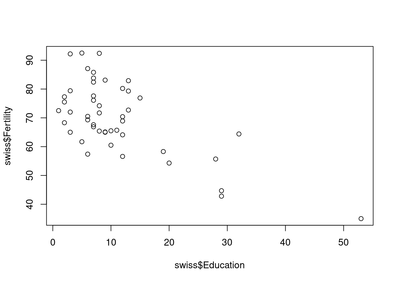
We use the classic `swiss` dataset from R, which includes a fertility measure and socio-economic indicators for 47 French-speaking provinces of Switzerland in 1888. The key variables for our analysis are **Fertility** (a standardized fertility measure) and **Education** (percentage of draftees with higher education). 


::: {.cell}

```{.r .cell-code}
summary(swiss[c("Fertility", "Education")])
#    Fertility      Education 
#  Min.   :35.0   Min.   : 1  
#  1st Qu.:64.7   1st Qu.: 6  
#  Median :70.4   Median : 8  
#  Mean   :70.1   Mean   :11  
#  3rd Qu.:78.5   3rd Qu.:12  
#  Max.   :92.5   Max.   :53
```
:::


*Table 1*. Summary of fertility and education in the `swiss` data (min, median, mean, max):


::: {#tbl-summary .cell tbl-cap='Descriptive statistics for Fertility and Education in 47 Swiss provinces (1888).'}
::: {.cell-output-display}


|   |Fertility    |Education  |
|:--|:------------|:----------|
|   |Min.   :35.0 |Min.   : 1 |
|   |1st Qu.:64.7 |1st Qu.: 6 |
|   |Median :70.4 |Median : 8 |
|   |Mean   :70.1 |Mean   :11 |
|   |3rd Qu.:78.5 |3rd Qu.:12 |
|   |Max.   :92.5 |Max.   :53 |


:::
:::


# Analysis

We first visualize the relationship between education and fertility (Figure 1).


::: {.cell}

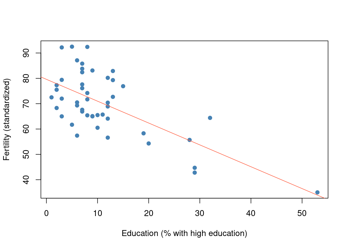
```{.r .cell-code}
plot(swiss$Education, swiss$Fertility,
     xlab="Education (% with high education)", ylab="Fertility (standardized)",
     pch=19, col="steelblue")
abline(lm(Fertility ~ Education, data=swiss), col="tomato")
```

::: {.cell-output-display}
![Scatterplot of Education (%) vs. Fertility (standardized) in Swiss provinces.](chapter1_files/figure-html/fig-scatter-1.png){#fig-scatter width=100%}
:::
:::


Figure @fig-scatter suggests a negative relationship – provinces with higher education levels tend to have lower fertility. To quantify this, we fit a simple linear model:


::: {.cell}

```{.r .cell-code}
model <- lm(Fertility ~ Education, data = swiss)
summary(model)
# 
# Call:
# lm(formula = Fertility ~ Education, data = swiss)
# 
# Residuals:
#    Min     1Q Median     3Q    Max 
# -17.04  -6.71  -1.01   9.53  19.69 
# 
# Coefficients:
#             Estimate Std. Error t value Pr(>|t|)    
# (Intercept)   79.610      2.104   37.84  < 2e-16 ***
# Education     -0.862      0.145   -5.95  3.7e-07 ***
# ---
# Signif. codes:  0 '***' 0.001 '**' 0.01 '*' 0.05 '.' 0.1 ' ' 1
# 
# Residual standard error: 9.45 on 45 degrees of freedom
# Multiple R-squared:  0.441,   Adjusted R-squared:  0.428 
# F-statistic: 35.4 on 1 and 45 DF,  p-value: 3.66e-07
```
:::


The model estimates that a 1% increase in education is associated with a decrease of -0.86 in the fertility measure on average. The relationship is statistically significant (< 0.001).

# Discussion

Our analysis finds an inverse correlation between education and fertility across Swiss provinces, consistent with the idea that more educated populations have lower fertility. This aligns with early observations of demographic transition (Notestein, 1945). Of course, this is a bivariate analysis; a deeper study might include other factors (e.g., economic indicators) and consider causality carefully. Nonetheless, it demonstrates the workflow: we obtained data, performed analysis, and generated a report with figures and references in a reproducible manner.

A few notes on the above content:

• We included a citation [@notestein1945]. Ensure refs.bib contains that key. We would add the Notestein reference (from 1945) in refs.bib manually or via Zotero. For example, in Zotero we find the reference (maybe a book chapter or article by Notestein) and use the citation picker to insert it. The extension would then add something like:

  @incollection{notestein1945,
    title = {Population: The Long View},
    booktitle = {Food for the World},
    author = {Notestein, Frank W.},
    year = {1945},
    publisher = {University of Chicago Press},
    address = {Chicago}
  }

  to refs.bib. We also set the style to APA, so it will format accordingly.

• We used a kable() from knitr to make a nice table of summary stats and gave it a label tbl-summary and a caption. Quarto will render that as a proper table with caption “Table 1” since we referenced it (I wrote “Table 1. …” manually above the table for clarity – Quarto doesn’t automatically number tables in text, so providing a label mainly helps cross-referencing within text, but numbering of tables in sequence will happen in the output).

• We created a plot and added a regression line. The fig-cap ensures it has a caption and number.

• We pulled out the p-value and coefficient from the model output inline, doing a little rounding/formatting in R within the backticks.

• The narrative describes what we did, referencing figure and theory.

Step 3: Render and refine. Save analysis.qmd. Now press Ctrl+Shift+K or run Quarto: Preview. The HTML preview appears. We scroll through it: the summary table is there, the scatterplot is shown as Figure 1 with its caption, the model summary is printed (which in HTML will be in a monospaced block). The citation appears as “(Notestein, 1945)” and at the bottom, a References section is created with the full reference. The reference is formatted in APA style (which in this case might look like: Notestein, F. W. (1945). Population: The Long View. In Food for the World. Chicago: University of Chicago Press.). Good – our Zotero integration and CSL are working.

We notice the scatterplot points are perhaps a bit small, maybe enlarge pch=19 was fine but color is nice. Suppose we want the regression line thicker. We can tweak the code: change abline(..., lwd=2). Hit save and preview again. The figure updates. We’re satisfied.

We also test PDF output: use Quarto: Render to PDF. A PDF is produced (assuming TinyTeX or equivalent is installed). We open it; everything is there with the same content. The figure is nicely included, and the References section is there in APA style. All good. If the PDF creation had an error (like missing LaTeX package), we’d fix that (TinyTeX usually minimizes such issues by including required packages on the fly).

Step 4: Using Git and GitHub. Now that our analysis is complete, we want to save our work in version control. In Positron, go to Source Control panel. We see analysis.qmd, refs.bib, and maybe analysis.html and analysis.pdf. Typically, you would version control the source (.qmd and .bib), and optionally the output. Including HTML/PDF in Git is sometimes avoided to keep the repo lightweight, but if it’s a small project, it’s fine. Let’s say we decide to include the HTML but not the PDF (because PDF can be binary and large). We add an entry in .gitignore for *.pdf. Now stage and commit:

• Stage analysis.qmd and refs.bib (click + on each).
• Commit with message: “Initial analysis report with data visualization and model.”
• Push to GitHub (if remote set). On GitHub, we can view the .qmd (as raw text) and the HTML if we push it could be viewed by enabling GitHub Pages or just manually.

For collaboration, if a colleague wants to contribute, they can clone the repo, open in Positron, and they have everything: the code, and by running Quarto they can regenerate the results. If they don’t have the packages installed, they’d install them (we could list them in README or use renv to lock them). They can also track changes via Git. If they add a new analysis or fix a bug, Git will show those changes.

Our entire workflow – from data to final document – is captured. Anyone can see how we got Figure 1, or what code produced the regression result, and the exact version of the source that produced the final output is in Git. This level of transparency is the goal of reproducible research.

Step 5: Using Zotero for a new citation (example extension in action). Imagine we want to cite another source, say an analysis from 2019 by Doe. We install the Zotero extension as described, press the hotkey, search “Doe 2019” and pick the reference. The extension inserts [@doe2019analysis] (for example) into our text and adds the entry to refs.bib. We render again, and we get a second reference listed, properly formatted. We commit the updated .qmd and .bib – now the history shows “added Doe 2019 citation”. If later we or someone else wonders “where did this statement come from?”, they see the citation and can find the source.

This example hopefully shows how Positron streamlines the development of a reproducible report. We wrote everything in one tool: code, text, formatting, references. We executed code and saw results immediately. We kept the project under version control, providing a safety net and collaboration mechanism. And we have a polished output that can be shared or submitted.

1.7 Best Practices for Reproducible and Collaborative Workflows

Using Positron with Quarto, Git, and Zotero provides a robust toolkit. However, tools alone don’t guarantee reproducibility – it’s how you use them. Here are some best practices to ensure your workflow remains reproducible, maintainable, and team-friendly:

• Literate Programming & Documentation: Write your analysis as a narrative. Don’t just show code and results; explain in prose what you’re doing and why. Quarto notebooks encourage this – use section headings, descriptive captions for figures and tables, and comments in code to clarify intent. Treat the Quarto document as both the analysis and the paper. This improves clarity and helps others (and future you) follow the logic. For example, rather than naming a section “Analysis 1”, name it “Regression of Fertility on Education” and explain the reasoning. Essentially, tell a story with your data.

• Modularize and Organize: If your project grows, consider splitting it into multiple files or using a Quarto project with chapters. Keep a logical folder structure: e.g., data/ for raw data, scripts/ for code experiments (if not all is in Quarto), results/ for output tables or figures (if you output them separately), and docs/ or report/ for the Quarto document(s). Positron (like VS Code) works with folders as “workspaces”, so leverage that structure for clarity. If using external data files, use relative paths in your code so that others can run the project by cloning the repo without having to modify paths. Quarto’s default working directory is the folder of the .qmd file (unless configured otherwise), so structure accordingly.

• Version Control Everything (and commit often): Make it a habit to commit your changes with meaningful messages. For instance, after writing the introduction, commit “Draft intro and background”. After adding a new analysis chunk, commit “Add regression analysis with output”. This granular history helps you later identify when results changed – e.g., “Oh, commit 5d2c1f8 updated the model to include an extra predictor, and that’s when Figure 2 changed.” It’s invaluable for back-tracking. Use branches for major changes or experimental ideas to avoid disrupting the main document until ready. Since Positron gives more control than RStudio’s simple Git GUI, you can do advanced Git operations easily – take advantage of that to maintain a clean history (squash commits if needed, revert problematic ones, etc.).

• Use Pull Requests for Collaboration: If working in a team, even if small, consider using GitHub pull requests for any changes to the main analysis. This provides an opportunity for peer review. A second set of eyes can catch errors or suggest improvements. Positron’s integration can make this smooth (you can review code side by side in the IDE). Tag each PR with what it’s about (e.g., “Improve data cleaning procedure”). Over time, the PR discussions serve as a record of why changes were made – useful for project memory.

• Environment Management: Ensure that anyone can install the required R packages and run the analysis. As mentioned, using renv to lock package versions is ideal for true reproducibility (so that, for example, if dplyr changes its API in a year, your project doesn’t break). If not using renv, at least document the R version and package versions you used (the sessionInfo() in an appendix trick, or a requirements.txt listing packages). This also includes recording other dependencies like having Python installed if you used it, or JAGS/Stan if doing Bayesian models, etc. Everything needed to get from data to results should be either in the code or documented.

• Seed Randomness: If your analysis involves random numbers (train/test splits, bootstrapping, etc.), set a set.seed() for reproducibility. Document it in your Quarto as part of the code. This way, someone rerunning your analysis will get the same “random” results. Otherwise, results might differ run-to-run, complicating verification.

• Use Plain Text Formats for Data When Possible: This is more data management, but if you have a choice, using CSV or TSV for data (instead of, say, Excel) is better for version control and transparency. You can diff and see changes in plain text. If data is large, consider not versioning it but rather provide a script to download or preprocess it. Or use Git LFS for large data.

• Leverage Quarto Project features: If your book or thesis has multiple chapters, Quarto can render an entire book (with cross-references across chapters). It can also create websites. Since this question is about a book chapter, note that Quarto Book format can automatically number chapters and sections, and aggregate references at the end, etc. Consider organizing chapters as separate .qmd files within a Quarto project for the whole book.

• Backup and Archive: In addition to GitHub (which is a cloud backup in effect), you might archive a snapshot of your project (especially upon publication of a paper or report) to a repository like Zenodo or OSF, which issues a DOI. This ensures long-term preservation. Journals often require data and code availability; a Quarto document plus data, archived, is a reproducible compendium of your research.

• Stay Current but Cautious: Keep an eye on updates to Positron, Quarto, R, and packages. Positron is evolving, and new features (or bug fixes) come often. For example, inline output or a package manager UI might appear in future versions. While writing your project, avoid updating critical components mid-stream unless needed (or unless you’ve locked versions). But do plan to update between projects to benefit from improvements.

By following these practices, you ensure that your analysis is not just a one-off result but a reproducible product. If someone asks, “How did you get Figure 3?”, you can point them to the exact code and data that produced it. If a collaborator or reviewer questions a step, you can show them the documented narrative and code in the Quarto report and even the commit history of how you refined that step. This level of transparency increases trust in your findings. It also makes your life easier in the long run – you can revisit the project after months and quickly recall what you did, and you can reuse pieces for other projects knowing the context in which they were developed.

1.8 Conclusion

Reproducible research in data science (and specifically in social sciences) is increasingly expected, and with modern tools it’s more achievable than ever. In this chapter, we demonstrated how Positron – a new IDE blending RStudio’s user-friendly features with VS Code’s flexibility – can serve as a one-stop platform for reproducible R research. We walked through setting up Positron with R and Quarto, noting that much of the configuration that VS Code required (installing extensions, etc.) is simplified in Positron’s integrated design. We saw that Positron supports R and Python out-of-the-box, so you can do multi-language work seamlessly, and it leverages the Visual Studio Code extension ecosystem via Open VSX (meaning you have a vast array of extensions at your disposal for extra functionality, from GitHub integration to Zotero citations, as we used).

Using a hands-on example, we showed how to integrate code and prose in a Quarto document, how to execute and refine analysis iteratively, and how to include references from Zotero easily. The output was a polished document with live code results and properly formatted citations – all generated with one click. This approach eliminates manual copy-paste of results and reduces errors, since the document is “single source of truth”: update the data or code, re-run, and the narrative and conclusions update accordingly if needed.

A key theme was version control with Git and GitHub. By versioning our project from the start, every change is tracked. When collaborating, this becomes the backbone of teamwork – enabling branching, pull requests, and peer review within the IDE. Positron’s interface makes these advanced practices accessible even to those who might shy away from the command line, which lowers the barrier to entry for researchers to adopt version control. We emphasized that even solo researchers benefit greatly from Git: it’s like an undo/redo for your entire project and a time machine to see how your analysis evolved. Plus, hosting on GitHub or similar platforms means your work can be open-source, inviting feedback and allowing others to learn from or build on it, which contributes to the scientific community.

For a graduate student or researcher used to “point-and-click” tools, transitioning to this workflow might seem daunting. But the learning curve is well worth it. Positron provides a gentle on-ramp: its RStudio-like layout feels familiar, so you can gradually incorporate VS Code-like enhancements (like extensions, advanced text editing, etc.) as you become comfortable. Meanwhile, Quarto as a modern rendition of R Markdown simplifies the creation of professional reports and even books or websites from the same material. It encourages good habits (like writing methods in-line with results, and citing literature properly). Zotero integration means you’re never manually formatting citations again – a huge time saver in thesis writing or literature-heavy fields.

By using these tools and practices, you’re not just aiming for reproducibility in a narrow sense (someone running your code on your machine gets the same result) – you’re aiming for true transparency and portability (someone else can take your code and data and get the same results on their machine, years later, and understand the process). This is the gold standard for computational research. It guards against errors (since analyses are documented and reviewable) and fosters trust in your conclusions. Moreover, it frees you from the fear of “what if I break something?” – because with version control and a script-based workflow, nothing is ever really lost and every change can be traced.

In closing, adopting a reproducible workflow with Positron, Quarto, Git, and Zotero turns your research projects into well-organized, traceable, and sharable projects. It might require adopting new habits (writing in source code vs. GUI, frequent committing, etc.), but once those habits form, you’ll likely find that you work more efficiently. No more scrambling to remember which file version had the final results, or which manual steps you did to clean the data – it’s all in the open. As you continue with this approach, you’ll also be aligning with the open science movement, contributing to a culture where research artifacts (code, data, methods) are as valued as the results themselves. This makes you a better collaborator and a more credible scientist.

References

• Andrew Heiss (2024). Fun with Positron. Heiss Blog. July 8, 2024. DOI: 10.59350/zs7da-17c67 .

• Jumping Rivers (2024). Positron vs RStudio – Is it time to switch? Jumping Rivers Blog (via R-Bloggers). December 4, 2024. .

• Matti Vuorre (2025). How to Add Citations from Zotero to Quarto Documents. Personal Blog. June 6, 2025. .

• Posit (2025). Positron Documentation – Remote SSH. Retrieved from Posit Docs (docs.posit.co). .

• Quarto Project (2025). Using Quarto with Positron. Quarto Documentation. .

• Appsilon (2023). Introducing Positron: A New, Yet Familiar IDE for R and Python. Appsilon Blog. .

• Posit Community (2023). Positron FAQ. (Information on extension support and differences from RStudio) .

• Marwick, B. (2016). Computational Reproducibility in Archaeological Research: Basic Principles and a Case Study of Their Implementation. Journal of Archaeological Method and Theory 24, 424–450. (Discusses principles of reproducibility in practice).

• Notestein, F. W. (1945). Population: The Long View. In Food for the World (pp. 36–57). Chicago: University of Chicago Press. (Classic reference on demographic transition theory referenced in text).