Chapter 1 Introduction
This course is part of the specialization in International Business. Like many academic disciplines, the field of international affairs benefits from the development of data science in order to formulate new quantitative approaches to the major themes of international affairs.
The objective of this course is to provide an introduction to the major themes of international business using different methods from data science. For example, how can data science be used to take a fresh look at global innovation? The use of APIs and data packets on innovation of multinational companies and on patents around the world will help answer this question. How can data science be used to analyze the global financial industry? How can data science be used to analyze the international business environment? How can data science be used to analyze global risks, such as the VIDOC-19 pandemic?
Throughout this course, students will learn and use the R language. This language will be complemented by the use of software suites such as Tableau, especially at the beginning of the course for data management. Packages of algorithms from reproducible research will also be used in R, such as TensorFlow. The learning of the R language and the various tools will be supported and reinforced by access to additional resources (data, courses, APIs, packets, etc.) made available on the course website.
In the end, students will be exposed to new methods made possible by recent advances in artificial intelligence analysis models, easy access to data in the field of international business and access to the necessary computing power.
Themes
Introduction to Data Science Methods for International Affairs
Use of useful data for international business
Use of algorithms applied to international business
Introduction to Machine Learning in the Context of International Business
Objectives
At the end of the course, the student will be able to:
Understand the usefulness of data science for the analysis of major international business issues;
Use data science and algorithmic formalization to solve international business problems;
Extract information relevant to decision making and risk analysis for international business;
Understand the important steps in building a predictive model;
Evaluate the performance of a predictive model;
Oral presentation of quantitative results and their interpretation;
Construct a report based on the principles of replicable research.
Pedagogical approach
The main pedagogical approach is that of reverse pedagogy based on the analysis of case studies. The content of the sessions will be known in advance and students should arrive prepared in class. Case studies will be used. An online multi-player simulation will be used in session 3. During each session, after a masterly presentation aimed at deepening the concepts and methods seen before the session, will follow an application work on a major theme of international affairs. For these topics, students will have access, for example, to databases on global patents, on all scientific articles on coronaviruses, on the most innovative multinational companies in the world, on the annual reports of the largest multinational companies, on Twitter conversations, etc. By using either structured or unstructured data, and combining this data with the appropriate models, students will be exposed to the new possibilities that are available to them.
Tools
Development tools: Table, R, RStudio, TensorFlow
Platform for interactive/online syllabus integrating code debugging, code teamwork, online quizzes, etc.; http://www.warin.ca
Simulation “World Health Organization: Data Science for Research against COVID-19”.
1.1 Course Material
https://towardsdatascience.com/all-machine-learning-algorithms-you-should-know-in-2021-2e357dd494c7
1.1.1 Linear Regression
Linear Regression is one of the most fundamental algorithms used to model relationships between a dependent variable and one or more independent variables. In simpler terms, it involves finding the ‘line of best fit’ that represents two or more variables.
The line of best fit is found by minimizing the squared distances between the points and the line of best fit — this is known as minimizing the sum of squared residuals. A residual is simply equal to the predicted value minus the actual value.
In case it doesn’t make sense yet, consider the image above. Comparing the green line of best fit to the red line, notice how the vertical lines (the residuals) are much bigger for the green line than the red line. This makes sense because the green line is so far away from the points that it isn’t a good representation of the data at all!
If you want to learn more about the math behind linear regression, I would start off with Brilliant’s explanation.
1.1.2 Logistic Regression
Logistic regression is similar to linear regression but is used to model the probability of a discrete number of outcomes, typically two. At a glance, logistic regression sounds much more complicated than linear regression, but really only has one extra step.
First, you calculate a score using an equation similar to the equation for the line of best fit for linear regression.
The extra step is feeding the score that you previously calculated in the sigmoid function below so that you get a probability in return. This probability can then be converted to a binary output, either 1 or 0.
To find the weights of the initial equation to calculate the score, methods like gradient descent or maximum likelihood are used. Since it’s beyond the scope of this article, I won’t go into much more detail, but now you know how it works!
1.1.3 K-Nearest Neighbors
K-nearest neighbors is a simple idea. First, you start off with data that is already classified (i.e. the red and blue data points). Then when you add a new data point, you classify it by looking at the k nearest classified points. Whichever class gets the most votes determines what the new point gets classified as.
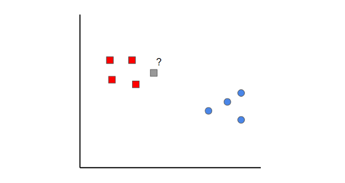
In this case, if we set k=1, we can see that the first nearest point to the grey sample is a red data point. Therefore, the point would be classified as red.
Something to keep in mind is that if the value of k is set too low, it can be subject to outliers. On the other hand, if the value of k is set too high then it might overlook classes with only a few samples.
1.1.4 Naive Bayes
Naive Bayes is a classification algorithm. This means that Naive Bayes is used when the output variable is discrete.
Naive Bayes can seem like a daunting algorithm because it requires preliminary mathematical knowledge in conditional probability and Bayes Theorem, but it’s an extremely simple and ‘naive’ concept, which I’ll do my best to explain with an example:
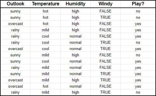
Suppose we have input data on the characteristics of the weather (outlook, temperature, humidity, windy) and whether you played golf or not (i.e. last column).
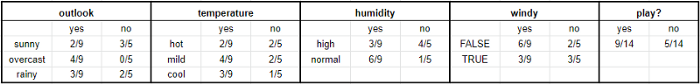
What Naive Bayes essentially does is compare the proportion between each input variable and the categories in the output variable. This can be shown in the table below.
To give an example to help you read this, in the temperature section, it was hot for two days out of the nine days that you played golf (i.e. yes).
In mathematical terms, you can write this as the probability of it being hot GIVEN that you played golf. The mathematical notation is P(hot|yes). This is known as conditional probability and is essential to understand the rest of what I’m about to say.
Once you have this, then you can predict whether you’ll play golf or not for any combination of weather characteristics.
Imagine that we have a new day with the following characteristics:
Outlook: sunny
Temperature: mild
Humidity: normal
Windy: false
First, we’ll calculate the probability that you will play golf given X, P(yes|X) followed by the probability that you won’t play golf given X, P(no|X).
Using the chart above, we can get the following information:
Now we can simply input this information into the following formula:
Similarly, you would complete the same sequence of steps for P(no|X).
Since P(yes|X) > P(no|X), then you can predict that this person would play golf given that the outlook is sunny, the temperature is mild, the humidity is normal and it’s not windy.
This is the essence of Naive Bayes!
1.1.5 Support Vector Machines
A Support Vector Machine is a supervised classification technique that can actually get pretty complicated but is pretty intuitive at the most fundamental level. For the sake of this article, we’ll keep it pretty high level.
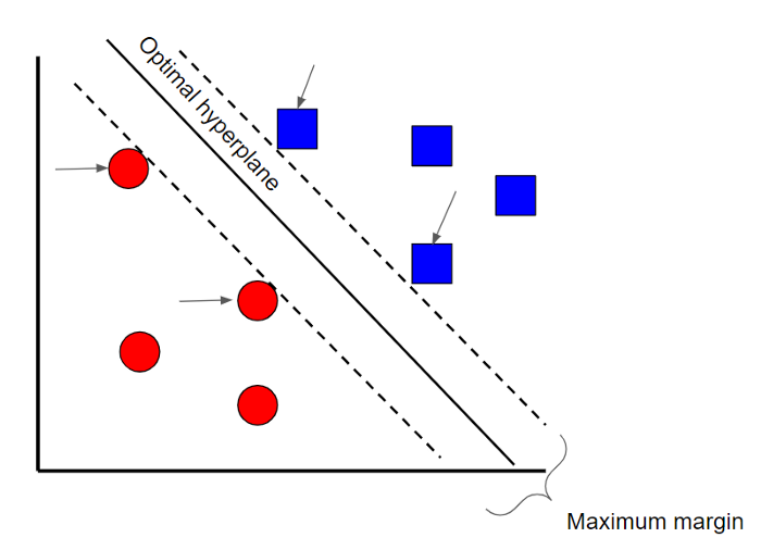
Let’s assume that there are two classes of data. A support vector machine will find a hyperplane or a boundary between the two classes of data that maximizes the margin between the two classes (see above). There are many planes that can separate the two classes, but only one plane can maximize the margin or distance between the classes.
If you want to get into the math behind support vector machines, check out this series of articles.
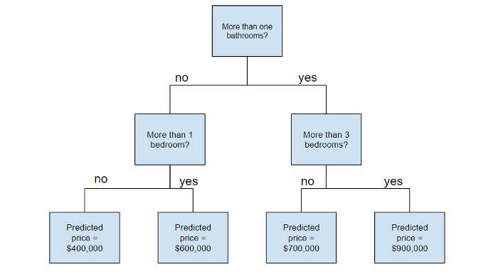
1.1.6 Decision Tree
1.1.7 Random Forest
Before understanding random forests, there are a couple of terms that you’ll need to know:
Ensemble learning is a method where multiple learning algorithms are used in conjunction. The purpose of doing so is that it allows you to achieve higher predictive performance than if you were to use an individual algorithm by itself.
Bootstrap sampling is a resampling method that uses random sampling with replacement. It sounds complicated but trust me when I say it’s REALLY simple — read more about it here.
Bagging when you use the aggregate of the bootstrapped datasets to make a decision — I dedicated an article to this topic so feel free to check it out here if this doesn’t make complete sense.
Now that you understand these terms, let’s dive into it.
Random forests are an ensemble learning technique that builds off of decision trees. Random forests involve creating multiple decision trees using bootstrapped datasets of the original data and randomly selecting a subset of variables at each step of the decision tree. The model then selects the mode of all of the predictions of each decision tree (bagging). What’s the point of this? By relying on a “majority wins” model, it reduces the risk of error from an individual tree.
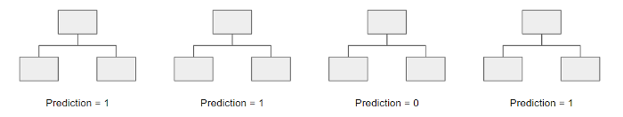
For example, if we created one decision tree, the third one, it would predict 0. But if we relied on the mode of all 4 decision trees, the predicted value would be 1. This is the power of random forests!
1.1.8 AdaBoost
AdaBoost, or Adaptive Boost, is also an ensemble algorithm that leverages bagging and boosting methods to develop an enhanced predictor.
AdaBoost is similar to Random Forests in the sense that the predictions are taken from many decision trees. However, there are three main differences that make AdaBoost unique:
First, AdaBoost creates a forest of stumps rather than trees. A stump is a tree that is made of only one node and two leaves (like the image above).
Second, the stumps that are created are not equally weighted in the final decision (final prediction). Stumps that create more error will have less say in the final decision.
Lastly, the order in which the stumps are made is important, because each stump aims to reduce the errors that the previous stump(s) made.
In essence, AdaBoost takes a more iterative approach in the sense that it seeks to iteratively improve from the mistakes that the previous stump(s) made.
If you want to learn more about the underlying math behind AdaBoost, check out my article ‘A Mathematical Explanation of AdaBoost in 5 Minutes’. Gradient Boost
It’s no surprise that Gradient Boost is also an ensemble algorithm that uses boosting methods to develop an enhanced predictor. In many ways, Gradient Boost is similar to AdaBoost, but there are a couple of key differences:
Unlike AdaBoost which builds stumps, Gradient Boost builds trees with usually 8–32 leaves.
Gradient Boost views the boosting problem as an optimization problem, where it uses a loss function and tries to minimize the error. This is why it’s called Gradient boost, as it’s inspired by gradient descent.
Lastly, the trees are used to predict the residuals of the samples (predicted minus actual).
While the last point may have been confusing, all that you need to know is that Gradient Boost starts by building one tree to try to fit the data, and the subsequent trees built after aim to reduce the residuals (error). It does this by concentrating on the areas where the existing learners performed poorly, similar to AdaBoost.
1.1.9 XGBoost
XGBoost is one of the most popular and widely used algorithms today because it is simply so powerful. It is similar to Gradient Boost but has a few extra features that make it that much stronger including…
A proportional shrinking of leaf nodes (pruning) — used to improve the generalization of the model
Newton Boosting — provides a direct route to the minima than gradient descent, making it much faster
An extra randomization parameter — reduces the correlation between trees, ultimately improving the strength of the ensemble
Unique penalization of trees
1.1.10 LightGBM
If you thought XGBoost was the best algorithm out there, think again. LightGBM is another type of boosting algorithm that has shown to be faster and sometimes more accurate than XGBoost.
What makes LightGBM different is that it uses a unique technique called Gradient-based One-Side Sampling (GOSS) to filter out the data instances to find a split value. This is different than XGBoost which uses pre-sorted and histogram-based algorithms to find the best split.
1.1.11 CatBoost
CatBoost is another algorithm based on Gradient Descent that has a few subtle differences that make it unique:
CatBoost implements symmetric trees which help in decreasing prediction time and it also has a shallower tree-depth by default (six)
CatBoost leverages random permutations similar to the way XGBoost has a randomization parameter
Unlike XGBoost however, CatBoost handles categorical features more elegantly, using concepts like ordered boosting and response coding
Overall, what makes CatBoost so powerful is its low latency requirements which translates to it being around eight times faster than XGBoost.