2 R for the impatient
This chapter serves as a quick-reference guide and learning bridge for students and professionals who are new to data analysis with R or Python, or transitioning between the two. It is intended to build foundational fluency in using both languages to manipulate data, generate descriptive statistics, and produce visualizations.
By the end of this chapter, you will:
- Understand the basic syntax and logic of R and Python for data analysis
- Learn equivalent commands between R and Python for common data tasks
- Be able to read and write small data workflows in both languages
- Appreciate the different programming paradigms and ecosystems of R and Python
- Cultivate good habits in coding, inspecting, and visualizing data
This chapter is especially designed to be hands-on and applied. It favors practical functionality over theoretical depth (which will come later). It can be revisited throughout the book as a reference when working through more complex statistical and machine learning models.
2.1 R and Python Command Reference Table
| Description | R Command | Python Equivalent |
|---|---|---|
| Obtain documentation | help() |
help(function_name) |
| View usage examples | example() |
import pydoc; pydoc.help() |
| Manually enter data | c(), scan() |
list(), input() |
| Create a sequence | seq() |
range(), numpy.arange() |
| Repeat values | rep() |
itertools.repeat() |
| Load built-in dataset | data() |
from sklearn import datasets |
| Spreadsheet view | View() |
df.head(), df.to_string() |
| Inspect structure | str() |
type(), df.info() |
| Read CSV file | read.csv() |
pandas.read_csv() |
| Load package | library() |
import module_name |
| Dataset dimensions | dim() |
df.shape |
| Vector length | length() |
len() |
| List objects in memory | ls() |
dir(), locals() |
| Remove object | rm() |
del object_name |
| Variable names | names() |
df.columns |
| Histogram | hist() |
matplotlib.pyplot.hist() |
| Lattice histogram | histogram() |
seaborn.histplot() |
| Stem plot | stem() |
matplotlib.pyplot.stem() |
| Frequencies | table() |
collections.Counter(), value_counts() |
| Cross-tabulation | xtabs() |
pandas.crosstab() |
| Mosaic plot | mosaicplot() |
statsmodels.graphics.mosaicplot() |
| Bin values | cut() |
pandas.cut() |
| Mean | mean() |
numpy.mean(), df.mean() |
| Median | median() |
numpy.median(), df.median() |
| Apply by group | by() |
df.groupby().apply() |
| Summary statistics | summary() |
df.describe() |
| Variance and SD | var(), sd() |
numpy.var(), numpy.std() |
| Sum values | sum() |
sum() |
| Quantiles | quantile() |
df.quantile() |
| Bar graph | barplot() |
matplotlib.pyplot.bar() |
| Lattice barplot | barchart() |
seaborn.barplot() |
| Boxplot | boxplot() |
matplotlib.pyplot.boxplot() |
| Lattice boxplot | bwplot() |
seaborn.boxplot() |
| Scatterplot | plot() |
matplotlib.pyplot.plot(), seaborn.scatterplot() |
| Lattice scatterplot | xyplot() |
seaborn.relplot() |
| Linear regression | lm() |
statsmodels.api.OLS(), sklearn.linear_model.LinearRegression() |
| ANOVA | anova() |
statsmodels.api.anova_lm() |
| Predictions | predict() |
model.predict() |
| Non-linear fit | nls() |
scipy.optimize.curve_fit() |
| Model residuals | residuals() |
model.resid |
| Sampling | sample() |
random.sample(), df.sample() |
| Repeat process | replicate() |
list comprehension, numpy.tile() |
| Cumulative sum | cumsum() |
numpy.cumsum() |
| Empirical CDF | ecdf() |
statsmodels.distributions.ECDF() |
| Binomial distribution | dbinom() |
scipy.stats.binom |
| Poisson distribution | dpois() |
scipy.stats.poisson |
| Normal distribution | pnorm() |
scipy.stats.norm |
| Student t-distribution | pt() |
scipy.stats.t |
| Chi-square | pchisq() |
scipy.stats.chi2 |
| Binomial test | binom.test() |
scipy.stats.binom_test() |
| Proportion test | prop.test() |
statsmodels.stats.proportion.proportions_ztest() |
| Chi-square test | chisq.test() |
scipy.stats.chi2_contingency() |
| Fisher’s test | fisher.test() |
scipy.stats.fisher_exact() |
| Student t-test | t.test() |
scipy.stats.ttest_1samp(), ttest_ind() |
| Normal QQ plot | qqnorm() |
scipy.stats.probplot() |
| Add margins to table | addmargins() |
df.apply() with margins |
| Proportions from table | prop.table() |
df.div(df.sum()) |
| Graphics parameters | par() |
matplotlib.rcParams |
| Power analysis | power.t.test() |
statsmodels.stats.power.tt_ind_solve_power() |
2.2 Pedagogical Notes
1. Learn by comparison: This chapter encourages “cognitive mapping” between languages. Comparing syntax fosters deeper structural understanding and strengthens both retention and flexibility.
2. Vocabulary building: Think of R and Python as two dialects of the same statistical language. Learning the synonyms improves fluency, especially when reading others’ code.
3. Practice matters: Run both versions of simple scripts. Use a dataset like iris, mtcars, or any CSV to experiment. Code repetition is key to internalizing patterns.
4. Expect asymmetry: Not all commands will have perfect equivalents. That’s part of the learning curve. Focus on what the function does, not just how it’s called.
2.3 Examples in R and Python
Load Data
# Python
import pandas as pd
mydata = pd.read_csv("https://example")
mydata.head()
mydata.shape
mydata.columns
Descriptive Statistics
# Python
mydata['hsgradrate'].mean()
mydata['hsgradrate'].median()
mydata['hsgradrate'].min()
mydata['hsgradrate'].max()
Histogram and Plot
# Python
import matplotlib.pyplot as plt
plt.hist(mydata['childpov'], bins=15, color='red', density=True)
plt.show()
plt.scatter(mydata['childpov'], mydata['hsgradrate'], color='red')
plt.show()
Arithmetic Operations
# Python
import math
8 + 3
27 / 5
math.cos(-math.pi)
abs(-2**3)
math.sqrt(4068289)
x = 8 + 3
y = 3
x + y
x * y
z = x * y
z
Z  # will error
Object Management
# Python
dir()
del y
dir()
Basic Stats on Vectors
# Python
import numpy as np
ourdata = np.array([-3,2,0,1.5,4,1,3,8])
len(ourdata)
ourdata[4]  # 0-indexed
np.mean(ourdata)
np.median(ourdata)
np.ptp(ourdata)
np.std(ourdata, ddof=1)
np.var(ourdata, ddof=1)
pd.Series(ourdata).describe()
Plotting
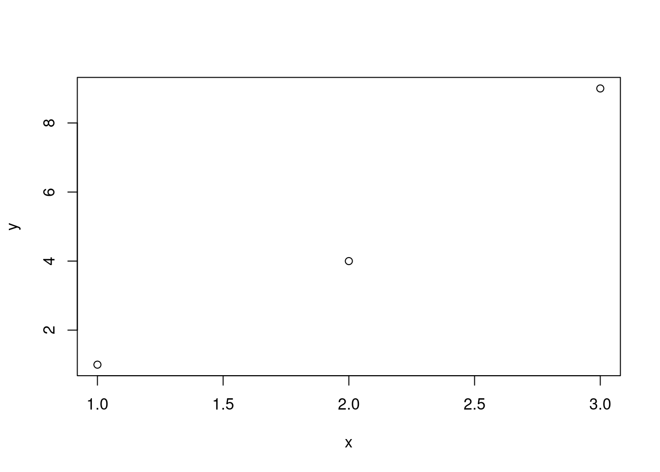
plot(x, y, xlab="x", ylab="y", pch=19, cex=0.8, col="blue", xlim=c(0,4), ylim=c(0,10), main="Our First Plot!", sub="STAT 100")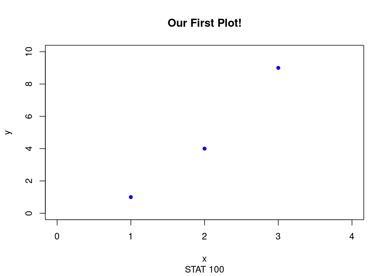
# Python
import matplotlib.pyplot as plt
x = [1, 2, 3]
y = [1, 4, 9]
plt.plot(x, y, 'bo-')
plt.xlabel("x")
plt.ylabel("y")
plt.xlim(0, 4)
plt.ylim(0, 10)
plt.title("Our First Plot!")
plt.suptitle("STAT 100")
plt.show()
Frequency Tables and Mosaic Plot
# R
table(mydata$childpov, mydata$hsgradrate)
xtabs(~hsgradrate, data=mydata)
xtabs(~hsgradrate + childpov, data = mydata)
mosaicplot(~hsgradrate + childpov, data = mydata)
# Python
import pandas as pd
pd.crosstab(mydata['childpov'], mydata['hsgradrate'])
pd.crosstab(index=mydata['hsgradrate'], columns='count')
pd.crosstab(mydata['hsgradrate'], mydata['childpov'])
from statsmodels.graphics.mosaicplot import mosaic
mosaic(mydata, ['hsgradrate', 'childpov'])
plt.show()