In this chapter, we will familiarize you with the essential tools for a reproducible data science workflow: the RStudio integrated development environment (IDE), the R Markdown document format, version control with Git and GitHub, and reference management with Zotero. These tools working together will allow you to easily create data analysis reports that integrate code and results, collaborate with others, and ensure your work is transparent and up-to-date.
RStudio is more than just a code editor – it provides a unified interface to write and run code (in R, Python, and more) and to compile documents. R Markdown is a simple formatting language that lets you combine prose, code, and results in one place. Git is a version control system that keeps track of changes to your files and facilitates collaboration via platforms like GitHub. Finally, reference management tools like Zotero, combined with RStudio add-ins, allow you to cite sources and automatically generate bibliographies in your reports. Mastering these will greatly enhance your efficiency and the reproducibility of your work.
At the end of this chapter, you should be able to:
Understand what an IDE is and recognize the key features of the RStudio IDE.
Create an account on RStudio Cloud (Posit Cloud) and set up a new RStudio project.
Navigate the RStudio interface, knowing the purpose of each of its four panels.
Create and save your first R Markdown document in RStudio and compile (knit) it to produce a report.
Understand the basics of Markdown syntax in R Markdown, including YAML headers, text formatting, code chunks, inline code, embedding images, and writing equations.
Explain the importance of Git for version control and collaboration, and use GitHub to host a project repository.
Link an RStudio project with a GitHub repository and perform the typical Git workflow: Pull, Commit, and Push changes.
Apply a consistent file naming convention (e.g., lowerCamelCase) for your project files.
Use Zotero (with the Better BibTeX extension) to manage references, and configure an R Markdown document to use citations.
Insert citations into your R Markdown document using the citr add-in and understand the syntax for citations if the add-in is not available.
Compile a bibliography in your report and ensure all cited sources are properly listed.
Throughout this chapter, tips and important points will be emphasized in bold or italics to catch your attention.
3.1 RStudio IDE and RStudio Cloud
RStudio is an example of an Integrated Development Environment (IDE). An IDE provides a graphical interface where you can write code, execute it, and manage the resulting output and files, all in one place. In simpler terms, an IDE connects your point-and-click actions to underlying commands (often the same commands you could run in a terminal) and organizes your workflow. Many IDEs exist, but RStudio is unique in how seamlessly it integrates multiple languages (R, Python, SQL, Markdown, and more) and tools for data science into a single cohesive environment. It lowers the barriers to entry for programming by providing an approachable interface without sacrificing power. In RStudio, a new user can easily mix narrative text and code to produce a report, while an advanced user can harness a full range of coding tools, all within the same window.
Even if you consider yourself a command-line expert, RStudio’s interface can boost your productivity by simplifying tasks (like plotting, debugging, or version control) that would otherwise require remembering complex commands. RStudio (developed by Posit, PBC) has undoubtedly helped broaden access to data science, enabling more people to participate in the so-called fourth industrial revolution of data and AI by making powerful tools more accessible.
This book is hands-on. We encourage you to follow along by actually clicking buttons and typing commands in RStudio to experience the process first-hand. Our focus is on the early stages of a data pipeline: from getting data into a data frame (a tabular data structure in R, akin to a spreadsheet) to organizing and visualizing data, and finally creating a business-oriented report or dashboard. We will not delve into advanced statistical modeling here, but by the end of these chapters you will have a solid understanding of how to build a reproducible data analysis workflow.
To get started, we will use RStudio Cloud, a cloud-based instance of RStudio that runs in your web browser. (Note: RStudio Cloud has been rebranded as Posit Cloud, but the functionality remains the same. We will refer to it as RStudio Cloud here.) Using RStudio Cloud means you don’t have to install anything on your computer initially, and you can access your RStudio environment from any machine with internet access. Later, if you prefer or require, you can install R and RStudio Desktop locally; however, the cloud version ensures everyone has the same setup during learning.
Setting Up an RStudio Cloud Account and Project
Follow these steps to create a free RStudio Cloud account and start a new project:
Create an account on RStudio Cloud: Open your web browser and go to https://rstudio.cloud/. Click on the “GET STARTED FOR FREE” button.
Click on the “Sign Up” button.
You will be presented with options to sign up. You can sign up using a Google account, GitHub account, or an email address. Choose whichever method you prefer and complete any required registration steps (such as verifying your email).
Create a New Project: Once logged in to RStudio Cloud, you will see a dashboard. Click on the “New Project” button to create a new RStudio project space.
After a moment, you should see a screen that allows you to configure the new project. You can generally accept the default settings here. The project will be provisioned (this may take a minute as a container with RStudio is started for you).
Create a new R Markdown file: Within your new RStudio Cloud project, you’ll be presented with the RStudio IDE interface (which we will describe in detail shortly). To start writing a report, create an R Markdown file. Click on the green “+” button at the top-left of the interface (this button creates a new file), and from the dropdown choose “R Markdown…”.
A dialog window may appear asking if you want to install necessary packages for R Markdown (if this is your first time using it on the project). Click “Yes” to install any required packages.
After a brief pause (while the system installs packages), another dialog window will appear titled “New R Markdown”. Here you can set a title and author for your new document. For now, you can leave the defaults or enter a sample title (e.g., “My First Report”) and your name as the author. Ensure the default output format is HTML. Then click “OK”.
RStudio will now open a new file tab in the top-left panel with some example content (this is a template R Markdown document). Before we proceed, save this file to your project. Click the floppy disk icon (💾) or press Ctrl+S (Windows/Linux) or Cmd+S (Mac).
When prompted, give the file a name (for example, “first_document.Rmd”) and confirm the save. Use a name without spaces or special characters (R Markdown files should have the extension .Rmd).
The new .Rmd file will now appear in the Files pane (usually the bottom right panel in RStudio). You have successfully created and saved an R Markdown document in your RStudio Cloud project.
At this point, you have an RStudio Cloud account and a project with a simple R Markdown file ready to go. Next, we will take a closer look at the RStudio IDE interface and learn what each part of the screen is for.
Understanding the RStudio Interface
When you open a project in RStudio (whether via RStudio Cloud or the desktop version), the interface is typically divided into four panels plus a menu toolbar. Each panel has a specific purpose and knowing what each one does will make you comfortable navigating RStudio as you develop your report.
Think of RStudio as analogous to a suite like Microsoft Office, but all integrated into one window. In one part of the screen you might be writing text (like in Word), in another you might be viewing data (like in Excel), and in another you could be typing commands (like a terminal). The difference is that in RStudio these components talk to each other fluidly. For instance, you can run a snippet of code and immediately see the result (a table or a chart) in another panel. Moreover, every time you re-run or compile your R Markdown document, you regenerate the analysis with the latest data and code, ensuring your report is always up-to-date.
Let’s break down the components of the RStudio interface (assuming the default layout):
Top Left Panel: Source Editor
The top left panel is the Source Editor. This is where you write your scripts and documents. In our case, this is where you will write your R Markdown document (with both text and code). You can think of this area as your text editor or word processor that has programming superpowers. For example, the content of this book was written in the R Markdown source editor panel of RStudio.
In the editor, you can have multiple tabs open (for multiple files). By default, when we created the new R Markdown file, it opened in a tab here. The content is color-coded for easier reading (for instance, R code might be colored differently than plain text).
At the top of this panel, there are a few important buttons:
The Save button (floppy disk icon) saves the current file. Remember to save frequently, especially before trying to run or knit your document.
The Knit button (blue icon with a ball of yarn or a circle – it might look like a ball of yarn or a cogwheel depending on your RStudio version) is used to compile your R Markdown document. We often call this “knitting” the document. Pressing Knit will tell RStudio to execute all the code in your R Markdown file and produce a formatted output document (by default, an HTML file).
When you click Knit, RStudio will ask you to save the file (if you haven’t already) and then it will run through the document. If all goes well, a preview of your compiled document will appear (often in a pop-up window or in a viewer panel). For an HTML output, RStudio will either show it in its Viewer or open it in your web browser. The compiled document will include all your text, as well as the results of any code (e.g., charts, tables) inserted in the appropriate places.
Another useful button in the editor toolbar is the Document Outline (it looks like a split rectangle or a bullet list icon). Clicking this toggles an outline view of your document (usually appearing in a pane on the left of the editor). This outline is basically a table of contents for your document, listing all the headings and subheadings. This is very handy for navigation as your documents grow longer – you can click on a section title in the outline to jump directly to that part of the document in the editor.
Bottom Left Panel: Console and Terminal
The bottom left panel is primarily the Console. This is where R commands are executed and results printed. When you click Knit to compile your document, you will see RStudio working through each step in the Console, and any messages, output, or errors will appear here. You can also type commands directly into the console prompt > to execute R (or Python, etc., if configured) commands interactively.
In the context of knitting an R Markdown document, the console will show you progress and any errors/warnings. For example, if your code has a mistake that causes the document to fail to compile, a red error message will appear in this panel, helping you diagnose the problem. If the document compiles successfully, the console will list the files that were created (for instance, it might say something like “Output created: first_document.html”).
The bottom left panel may have multiple tabs aside from the Console. By default, you might also see a Terminal tab (which gives you access to a shell command line, if needed) and a Jobs tab (for background tasks). For most of our needs, you will be looking at the Console tab in this panel.
Top Right Panel: Environment and Git
The top right panel serves a couple of purposes, primarily data and variable management, and version control. By default, it opens to the Environment tab.
Environment Tab: This tab lists all the R objects (data frames, variables, functions, etc.) that are currently loaded in your R session. When you load a dataset or create a new variable in your code, you will see it show up here. It’s like your workspace browser. This gives you a quick way to inspect what data you have in memory. For example, if you read a CSV file into a data frame called salesData, once that code runs, you’ll see an entry for salesData in the Environment tab along with some details like its type and dimensions. You can click on a data frame in the environment to open it in a spreadsheet-like view for a quick look at the data.
The Environment tab also has an Import Dataset button. This provides a GUI wizard to load data (from text files, Excel sheets, etc.) into R without writing code manually. Clicking this will help you browse for a file and set options (like whether the first row is a header, what the field separator is, etc.) and then import it, generating the corresponding R code for you. While we will teach you how to read data with code (which is more reproducible), this tool can be convenient for quick tasks or for beginners.
If you click Import Dataset, a dialog will appear where you can select the file and adjust settings. For example, you might choose a CSV file, specify that it’s comma-separated, and indicate that the first row contains column names. RStudio will then read the data and show you a preview. When you confirm, it will load the data into your environment (and you’ll see the data frame listed in the Environment tab).
Make sure to choose the appropriate settings when importing data: the delimiter (comma, semicolon, tab, etc.), whether the first row is a header (variable names) or actual data, how decimal points are represented, etc. Getting these right ensures your data is read correctly. (We will explore data importing and wrangling in detail in later chapters.)
After importing, if you click on the name of the dataset in the Environment tab, RStudio will open a viewer (usually in the top left panel) showing the first portion (up to 1,000 rows) of the data in a spreadsheet-like format.
Git Tab: Next to the Environment tab, you may see a Git tab (this will appear if your project is initialized as a Git repository; we will do this soon when we discuss Git). The Git tab will show version control information: which files have been modified, which are staged to commit, etc. From this tab, you can perform Git operations like commit, push, and pull through the RStudio interface. We will cover the specifics in the Git section of this chapter. For now, just note that this is where Git-related info lives in the RStudio interface.
There may also be a History tab in this panel, which logs the commands you have executed in the console.
Bottom Right Panel: Files, Plots, Packages, Help, and Viewer
Finally, the bottom right panel is a multipurpose area. By default, it opens to the Files tab, which shows the files and folders in your project’s working directory (essentially a file browser, similar to Finder on Mac or Explorer on Windows, but limited to your RStudio project directory).
Files Tab: This is where you can see all files associated with your project. You can navigate through sub-folders, and use the buttons provided to manage files. For instance, you can create a New Folder, upload or export files, or delete files. If you select a file, you can use the More button (with a gear icon) for additional options like renaming or moving it. One important option here is “Set As Working Directory” which tells R (and RStudio) to treat that folder as the base location for relative file paths. By default, when you open an RStudio project, the working directory is set to the project directory, so you usually won’t need to change it. (In our image examples, you might see a working directory path like askHector, which was an example project name – the notation ./ in front of paths indicates the current working directory.)
When working with R Markdown, it’s good practice to keep your data and images within your project and refer to them with relative paths (like ./data/mydata.csv or ./images/plot1.png). The Files tab helps you figure out those paths and manage your project’s content.
For example, if you have a subfolder called images and inside it an image diagram.png, the relative path might be ./images/diagram.png. We use this path when embedding images in our R Markdown to tell RStudio where to find the file.
Plots Tab: Whenever you generate a plot in R (for instance, by calling a plotting function in the console or in a code chunk and running it), it will appear under the Plots tab in this panel. You can navigate through previous plots using arrows, zoom into a plot, or export it (save as an image or PDF) from this tab.
Packages Tab: This shows a list of R packages installed in your environment, with checkmarks for those that are currently loaded. You can install new packages or update packages using the buttons here, but often it’s just as easy to use install.packages("packagename") in the console. Still, the Packages tab provides a quick way to attach a package (by checking its box, which runs library(packagename) for you) or see what version is installed.
Help Tab: If you use R’s help system (for example, ?mean or help(mean) in the console to get documentation on the mean function), the documentation will appear in the Help tab. It’s essentially a built-in web browser for R’s help files and any other documentation you open.
Viewer Tab: RStudio has an internal viewer for web content. When you create interactive plots (with packages like plotly or leaflet) or if you preview an HTML widget or a Shiny app, it might appear in the Viewer tab. Also, when you knit an R Markdown to HTML, by default RStudio might show it in this Viewer instead of your external web browser.
Think of the bottom right panel as your miscellaneous toolbox: file manager, plot viewer, package manager, help browser, etc., all in one.
As an example of using the Files tab, consider the path example from above. We mentioned an image with path ./R1images/bottomRightPanel.png in a description. That path indicates there is a folder named R1images in the current project, and inside it a file bottomRightPanel.png. Knowing how to read and use such paths is important when you link resources in your R Markdown (like including images or data files). The Files pane can help you verify those file names and paths.
In the Files pane, you have controls to manipulate files:
New Folder button: create a new directory in your project.
Upload (in RStudio Cloud or if enabled): bring files from your local system into the project.
More (gear icon): contains options to Rename, Delete, or Export (download) selected files, and as mentioned, Set As Working Directory which changes R’s reference point for relative paths.
Generally, you won’t need to set the working directory manually if you stick to using RStudio Projects, because the project’s main directory is automatically the working directory.
Primary Toolbar and Menus
At the very top of RStudio (above all panels) is the primary menu bar and toolbar. This includes menus like File, Edit, Code, View, Plots, Session, Build, Git, Tools, Help (these may vary slightly if using RStudio Desktop vs Cloud). Many of the functions accessible through buttons in the panels are also available via these menus.
Key items include:
File menu: Create new files, open recent projects, save files, etc.
Edit menu: Text editing functions (undo, copy, paste, find/replace, etc.).
Run menu (or on toolbar): Buttons to run code from the source editor (like running the current line or selected code, which sends it to the Console).
View: Options to zoom or rearrange panels.
Session: Controls for your R session (restart R, interrupt running code, set working directory, etc.).
Git (if a Git repo): Quick access to version control operations.
Tools: Global options, addins, managing packages, etc.
Help: Access documentation and diagnostics.
In addition to menus, the toolbar typically has icons for common actions (New file, Open file, Save, Knit, Run, etc.). We will explore certain toolbar features (like Addins) later in this chapter when we discuss the citr add-in for citations.
To go further: If you want to set up R and RStudio on your own computer (instead of or in addition to using RStudio Cloud), there is a tutorial available that walks through installing R, RStudio, and necessary packages. You can refer to this guide for detailed steps on local installation and configuration.
TL;DR – RStudio Interface Overview:
IDE (Integrated Development Environment): A software application (like RStudio) that provides comprehensive facilities to programmers for software development, combining a source code editor, build automation tools, and more, in one GUI.
RStudio environment is split into four main panels:
Top Left (Source Editor): Where you write your text and code (R scripts, R Markdown files, etc.). This is your main coding area with a text editor and action buttons like Save and Knit.
Bottom Left (Console/Terminal): Where code runs and output or error messages appear. You can also type commands here directly. It shows the log and progress when knitting documents.
Top Right (Environment/History/Git): Shows your data and variables in the Environment tab. Also includes the Git tab for version control (when using Git) and can show command history.
Bottom Right (Files/Plots/Packages/Help/Viewer): A multipurpose area for browsing project files, viewing plots, managing packages, reading help files, and previewing web content or reports.
By understanding what each panel does, you can efficiently navigate RStudio and make the most of its features while developing your data analysis projects.
Thanks! I’ll retain the R Markdown material as-is, then add a new section introducing Quarto (.qmd), including its differences from R Markdown, advantages, and the ability to use other languages like Python or Julia in code chunks. I’ll let you know as soon as that section is ready.
3.2 Writing Documents with R Markdown (and Quarto)
Now that you have set up the RStudio environment, let’s focus on creating content using R Markdown. (We will also introduce Quarto, a newer system similar to R Markdown, later in this section.) R Markdown is one of the two main tools we will use throughout this book (the other being R itself). It allows you to combine regular text (formatted in a simple, readable way) with chunks of R code. When you knit an R Markdown document, the code is executed and its output is embedded in the final document, which can be rendered to various formats like HTML, PDF, Word, or even presentation slides.
Using R Markdown is central to the concept of reproducible research: your report is reproducible because anyone with your R Markdown file and data can re-run it to get the same results. If the data are updated or the analysis needs to change, you edit the code in one place (the R Markdown file) and knit again to produce an updated report. This is much more efficient and less error-prone than manually updating numbers or plots in a Word document.
In this section, we will create a simple R Markdown document and learn the basics of the Markdown syntax and structure. (If you followed the steps in the RStudio Cloud setup, you have already created an R Markdown file with a sample template. We will use that as a starting point. If not, here is how you can create a new R Markdown document in any RStudio session.)
Creating a New R Markdown Document
To create a new R Markdown document in RStudio, use the menu: File > New File > R Markdown…. This will open a dialog for specifying the title, author, and output format of your new document.
Choose Document (the default) as the type of R Markdown (as opposed to Presentation or other specialized formats) and ensure the default output is HTML. Enter a title and author if you’d like (you can change these later in the document’s YAML header). Then click OK.
RStudio will create a new file (with some example content) and open it in the source editor. Don’t forget to save this file (with a name ending in .Rmd). Once saved, you can proceed to edit the content.
At this point, if you have been following along, you should have achieved a couple of things already:
Familiarized yourself with the RStudio IDE layout.
Created (and saved) your first R Markdown document in RStudio.
Now we will dive into how to write in R Markdown.
The Structure of an R Markdown Document
An R Markdown document has three basic components:
The YAML header at the very top (optional but important for specifying document metadata and output options).
The body of the document, which includes your narrative text mixed with code chunks that execute R (or other languages’) code.
(Possibly) a section for references at the end, if you are citing sources (we will cover citations later).
Let’s go through these components and some key syntax elements of Markdown.
YAML Header
YAML stands for “YAML Ain’t Markup Language” (a recursive acronym) – essentially, it’s a human-readable format for specifying configuration. In an R Markdown file, the YAML header is the section at the very top enclosed by triple dashes --- at the beginning and end. It provides metadata about the document and instructions for the output format.
Here’s an example of a simple YAML header in an R Markdown (.Rmd) file:
---title:"My First Report"author:"Jane Doe"date:"26/06/2025"output: html_document---
This YAML header specifies:
title: The title of the document (appears at the top of the report).
author: The author name (appears below the title in many formats).
date: The date (or any text you want in the date field).
output: The output format. Here html_document means we want to knit to an HTML file. Other common options include pdf_document for PDF output, word_document for a Word .docx file, beamer_presentation for a PDF slide deck, ioslides_presentation for HTML slides, and github_document for a Markdown output suitable for GitHub. You can change this depending on what final format you need.
You can add many other options in YAML. For example, toc: true will include a table of contents, bibliography: references.bib can specify a file for references (useful when you need to cite sources), or you can specify visual themes for slides and documents. In our simple documents, we’ll often stick to just the basic fields shown above.
The YAML header is incredibly convenient because it lets you switch the entire output format or other settings without touching the main body of your document. For instance, if you wrote a report and later need it as a presentation, you can change output: html_document to output: ioslides_presentation (and maybe tweak a few things in the content) and knit again to get slides. The same content can be output in different forms with minimal effort.
One thing to note: If you are used to word processors, you might be tempted to adjust the formatting of specific sections manually (like making one heading a different color or a specific line a larger font). In R Markdown (and Quarto), a lot of that fine-grained control is handled by the output format’s template or by using custom CSS/LaTeX templates, rather than in the document content itself. The idea is that you focus on content, and let the template handle the style. This can be a mental adjustment: you give up a bit of immediate control over appearance in exchange for consistency and speed. The upside is huge – you won’t spend time tweaking formatting on every update, and your documents will have a professional, consistent style. The downside is you may need to learn a bit about styling (CSS or LaTeX) if you want to customize beyond the provided templates, but for most cases you can find a template or default that looks good.
(If you ever need to highly customize appearance, you can. But as a tip: content is king. It’s often better to use the default styles unless you have a compelling reason – they are usually chosen by experts in design to be clean and readable.)
R Code Chunks
The real magic of R Markdown is its ability to run code and insert the results into the final document. This is done with code chunks. A code chunk in R Markdown looks like this in the source:
::: {.cell}

```{.r .cell-code}
# This is an R code chunk
summary(cars)
```
:::
Everything between the ```{r} and the closing ``` is interpreted as R code (not as text for the report). When you knit the document, that R code will be executed. Anything the code prints to output (like the summary of a dataset, or a plot) will be captured and inserted into the document at that position.
Here, cars is a built-in dataset in R (a simple data frame of car speeds and stopping distances). summary(cars) will produce summary statistics for each column (min, max, mean, etc.). When you knit the document, those statistics will appear in the output at the position of the chunk.
If you have multiple lines of code in one chunk, they will all run in sequence. You can also include comments in your code (lines starting with #), which are ignored by R when running. Comments in code chunks will not appear in the output document (they’re not text for the report, just notes to yourself in the source).
This chunk, when run, will produce a scatter plot of the cars dataset (speed vs stopping distance), and that plot image will be inserted into the document.
By default, code chunks will also echo the code (show the code itself) in the output document, followed by the results or plot. However, you can control chunk behavior with chunk options inside the curly braces { } that start the chunk. For example:
{r, echo=FALSE} – runs the code without showing the code in the output (only the results will appear).
{r, include=FALSE} – runs the code but includes neither the code nor the results in the output (useful if you need to set something up in code that the reader doesn’t need to see).
{r, eval=FALSE} – shows the code in the output but does not actually execute it (useful for showing code examples without running them).
There are many such options (like controlling figure size, whether to cache results for speed, etc.), but we won’t overwhelm you with those now. The default behavior is usually fine for learning purposes.
In RStudio’s editor, you can also run individual chunks without knitting the whole document by clicking the little green triangle “play” button that appears to the right of a chunk, or by using the shortcut Ctrl+Shift+Enter (Windows) or Cmd+Shift+Enter (Mac) when your cursor is inside a chunk. This executes the chunk and shows you the output in the console or plot pane, which is handy for testing and iterative work.
Inline Code
Sometimes you want to embed a single value or a small result directly in your text, rather than showing it as a separate block. For example, you might want to write: “The average speed is 15.4 mph” where that number is calculated from data. Hard-coding such numbers in text is not reproducible (if the data updates, your text would be wrong unless you remember to update it too), but R Markdown allows inline code to solve this.
Inline R code is written using a single backtick ` followed by r and the code, then another backtick. For example: 15.4 in your text will be replaced by the result of the R expression mean(cars$speed) when the document is knit.
So you could write in your R Markdown file:
The average speed of the cars dataset is 15.4 miles per hour.
When you knit, that will become something like:
“The average speed of the cars dataset is 15.4 miles per hour.” (assuming 15.4 is the actual mean of that dataset).
Inline code is extremely useful for embedding statistics or results in your narrative. It ensures consistency between what your analysis calculates and what you describe in the text, because the value is generated dynamically. If your data changes or you do a different analysis, the narrative text will update on the next knit.
One thing to note: inline code should be brief. It’s not meant for long computations or producing plots; it’s for a single number or a short piece of text. Also, by default inline results are inserted as plain text (if they’re numeric, they’ll be formatted as numbers). You can control formatting (like number of decimal places) using R functions or formatting options if needed (for example, using the round() function inside the inline code to round a number).
Basic Markdown Syntax for Text
Now let’s cover how to format the text itself in your R Markdown document using Markdown syntax. Markdown is designed to be simple and readable as plain text, while allowing for basic formatting. Here are some common elements:
Headings: Use the # symbol to denote headings. The number of # you use indicates the level of the heading. For example:
# Heading 1 (usually the document title; if you use the YAML title, you typically don’t need to put a level-1 heading in the body).
## Heading 2 (a major section heading).
### Heading 3 (a subsection).
You can continue to smaller sub-sections with ####, #####, etc., but rarely do you need more than 3-4 levels in a short report.
In the output, these will be formatted with decreasing font sizes or emphasis. They will also be used to build a table of contents if you enabled toc: true in the YAML.
Bold and Italic text:
To make text bold, wrap it in double asterisks, like **this**, or in double underscores __this__.
To make text italic, wrap it in single asterisks *this* or single underscores _this_.
You can combine for bold and italic with triple asterisks/underscores, but that’s less common.
Lists:
Unordered lists (bulleted lists): Start a line with a dash - or an asterisk *. Indent by 2 spaces (or a tab) to create sub-lists. For example:
- First bullet item
- Second bullet item
  - Sub-item
  - Sub-item
- Third bullet item
will produce a bulleted list with a sub-list under the second item.
Ordered lists (numbered lists): Start lines with 1., 2., etc. The numbers will automatically display in order when rendered (you can actually just put 1. for each and Markdown will number them correctly).
1. Step one
2. Step two
3. Step three
will produce an ordered list of steps.
You can mix lists with paragraphs or sublists, but be careful with indentation so that Markdown knows what is part of a list versus a new paragraph.
Links: To insert a hyperlink, use the format [link text](URL). For example: [RStudio website](https://www.rstudio.com){target="_blank"} will render as a clickable link: RStudio website. (The {target="_blank"} part is optional; it makes the link open in a new tab for HTML output.)
Images: In Markdown, images are inserted similar to links but with an exclamation mark prefix. The syntax is . You can include alternative text inside the brackets for accessibility (in case the image doesn’t load). For example:
will include the image at that path, scaled to a width of 200 pixels (the {width=...} is a way to suggest a display width; it’s especially useful for LaTeX/PDF output for controlling image size). In our documents, we often provide images with a specific width for consistency.
In this chapter, we have an images folder in our project, and we reference images by their relative path. This keeps the document self-contained (as long as the images folder accompanies the document).
Code formatting in text: If you want to refer to a piece of code or a filename in your narrative (without executing it), you can format it as code by wrapping it in single backticks. For example, “Use the function mean() to calculate the average” or “Open the file analysis.Rmd for editing.” This will display the text in a monospaced font and distinguish it as code.
Blockquotes: If you want to quote a passage or provide a highlighted note, start the line with >. For example:
> Data science is the art of turning data into actions.
will appear as an indented block quote. (We won’t use blockquotes often for our purposes, but it’s good to know.)
These are the most frequently used Markdown elements for basic writing. There are others (like tables, which we’ll see later when discussing references and citations, or horizontal rules using --- or ***), but the above covers the essentials. You can always refer to the RStudio Markdown cheatsheet for a quick reference on syntax (R Markdown Cheat Sheet (PDF)).
Adding Mathematical Notation
If you need to include mathematical equations or symbols, R Markdown (via Pandoc’s Markdown) allows you to use LaTeX math notation:
For inline math, wrap the LaTeX in single dollar signs. Example:
The formula for the line is $y = \alpha_0 + \alpha_1 x_1 + \alpha_2 x_2 + \epsilon$.
This will render inline, for example: The formula for the line is \(y = \alpha_0 + \alpha_1 x_1 + \alpha_2 x_2 + \epsilon\).
For display (centered) equations that appear on their own line (typically numbered in scholarly writing), use double dollar signs on separate lines:
This will display the equation centered on its own line: \(y_i = \alpha_0 + \alpha_1 x_{i1} + \alpha_2 x_{i2} + \alpha_3 x_{i3} + \epsilon_i\)
You can include Greek letters (e.g., \alpha for α), subscripts with _ (e.g., x_{i1} for \(x_{i1}\)), superscripts with ^ (e.g., x^2 for \(x^2\)), fractions with \frac{a}{b}, summation symbols \sum, and so on. Essentially, anything you could write in LaTeX math mode can be done in R Markdown. This is extremely powerful for reports that include statistical or mathematical formulas.
Knitting the Document
Once you have some content in your R Markdown file – a combination of text, code chunks, etc. – you can generate the output by clicking the Knit button in RStudio. It’s the button with a ball of yarn icon and a needle, at the top of the source pane. If you’re not using RStudio, you can also knit by calling a function in R (e.g., rmarkdown::render("your_file.Rmd")), but in RStudio the button is easiest.
When you click Knit, RStudio will run through the document, executing each code chunk in a clean R session, capturing the output and plots, and then assembling everything into the final document (HTML, PDF, etc., depending on your YAML). If there are errors (for example, a chunk of R code has a mistake), the knitting process will stop and you’ll see an error message in the R console. You would then fix the issue and knit again. If all goes well, you’ll get an output document in your chosen format.
For example, if you knit the default sample R Markdown that RStudio created when you made a new file, you’ll get an HTML page with a title, some introductory text, a plot of the pressure dataset, and a few other examples. RStudio will likely open this in its Viewer pane (or you can open the HTML file in a web browser).
Every time you knit, you’re running a fresh execution of the document. That means it’s reproducible – the output document doesn’t rely on anything you did before by hand (you’re not copy-pasting results; the code in the document always generates the results from scratch). It also means that if you change the data or update a parameter in your analysis, those changes will be reflected the next time you knit. This ensures your report is always in sync with your latest analysis or data.
By this point, you should be comfortable creating an R Markdown file, writing basic content with Markdown formatting, and including R code to perform computations or generate plots. You should also be able to click Knit and produce a nicely formatted output document that combines text and code results.
Reproducible Research Note: We emphasize reproducibility because it saves time and avoids errors. For instance, imagine using R Markdown for a business report: next month you get new data, so you update the data file and re-knit the report. All the tables and figures update automatically based on the new data. Contrast this with a manual process (like updating numbers in Excel and copying them into Word) – that approach is tedious and prone to mistakes. Embracing tools like R Markdown means your work is not only more efficient for yourself, but also easier to hand off to someone else or to revisit after time, since everything needed to regenerate the results is in one place (the script and the data).
As a real-world example of reproducible research and transparency, consider an initiative in academia: many journals encourage or require authors to publish replication materials. For example, there is a repository of academic articles in economics where each paper’s data and code are made available so others can reproduce the findings. You can explore one such repository here: Economic Articles – Reproducible Research. This site lists economics papers that come with code and data, allowing anyone to rerun the analysis. It’s a good reminder of the growing expectation in many fields that results should be reproducible.
TL;DR – Key R Markdown Elements:
YAML header at the top (between --- lines) defines document title, author, date, and output format (among other options).
Write narrative text in Markdown: use # for headings, **bold** or *italic* for emphasis, - for bullet lists, 1. for numbered lists, etc.
This will run the code and include its output (or plot) in the document.
Include inline R code with `r` to insert computed values into your text.
Embed an image with Markdown syntax, e.g.  (optionally with size attributes like {width=400}).
Write equations with LaTeX syntax: $E = mc^2$ for inline or $$E = mc^2$$ for a standalone formula.
Click Knit to compile the document and see the output. If using a different environment, run the render function to produce the output file.
Some R functions we used in the examples above:
summary(object) – produces summary statistics of a dataset or R object.
plot(object) – produces a plot (the output depends on the type of object; for a data frame like cars, it will make a quick scatter plot).
mean(vector) – calculates the mean of a numeric vector.
Quarto (.qmd): A Modern Alternative to R Markdown
By the way, there’s a newer tool called Quarto that you might hear about. Quarto (with file extension .qmd) is essentially the next generation of R Markdown, introduced by Posit (formerly RStudio) in 2022. It extends the ideas of R Markdown to be multi-language and multi-engine. In practical terms, a Quarto document looks and feels very much like an R Markdown document: you write Markdown text, you include code chunks, and you render the document to formats like HTML, PDF, Word, slides, etc. The big difference is that Quarto isn’t limited to R – it allows you to use Python, Julia, JavaScript, and other languages in your code chunks, in addition to (or instead of) R.
If you are only using R, Quarto will behave almost identically to R Markdown for your purposes. In fact, Quarto can render most existing .Rmd files without modification. But Quarto provides a unified framework for doing more, and it’s likely to be the focus of new features going forward. Here, we’ll give a brief overview of Quarto and how it compares, so you’re aware of it.
Creating a New Quarto Document: To create a Quarto document in RStudio (version 2022.07 or later), you can use the menu File > New File > Quarto Document. This is analogous to creating an R Markdown file. When you do this, you’ll get a new file with extension .qmd. The RStudio IDE will recognize it as a Quarto file. The sample content of a new Quarto document is very similar to the R Markdown template, just with slight differences in the YAML and perhaps an example of a Python chunk. Don’t forget to save the file (with a .qmd extension).
The RStudio IDE shows a Render button (often a blue circle icon with a white “Q”) when you have a Quarto document open. This replaces the Knit button for .qmd files. Clicking Render will execute the Quarto workflow (which, behind the scenes, runs the code and uses Pandoc to create the output). The experience of writing and rendering is otherwise quite similar to R Markdown. You can also render Quarto documents from the command line using quarto render mydocument.qmd or from R by using the Quarto R package (quarto::quarto_render("mydocument.qmd")), but using the RStudio button is easiest when you’re working interactively.
Structure of a Quarto Document: A .qmd file also has three main parts, much like R Markdown:
A YAML header at the top (between --- lines) for title, author, output format, etc.
The body of the document with Markdown text and code chunks.
An optional references/bibliography section at the end (if you need to cite sources).
Everything you learned about writing Markdown text (headings, lists, bold/italic, links, images, etc.) and including mathematical notation applies equally to Quarto. The Markdown syntax is the same. The idea of code chunks is also the same, but with Quarto you are not restricted to R for those chunks.
YAML in Quarto: The YAML fields in a Quarto document are largely the same, but the output format is specified a bit differently. Instead of output: html_document (which was specific to the R Markdown system), Quarto uses format to specify output. For example, a simple Quarto YAML might be:
---title:"My First Report (Quarto)"author:"Jane Doe"date:"26/06/2025"format: html---
This tells Quarto to produce an HTML document. If you wanted a PDF, you would use format: pdf. For a Word document, format: docx. Quarto has short, intuitive names for formats (it consolidates what was a variety of output functions in R Markdown into a single system). You can even list multiple formats if you want to render to, say, HTML and PDF at the same time (Quarto can target multiple outputs in one render, using a list under format field). For example:
would produce both HTML and PDF outputs with one command. But for now, you can stick to a single format like HTML.
All the other YAML options (title, author, date, toc, etc.) work similarly in Quarto. In fact, you’ll often find that you can copy an R Markdown YAML header into a Quarto doc and just adjust the output/format field and it works.
Code Chunks in Quarto: Quarto’s code chunks are very flexible. You still delineate a code chunk with triple backticks and curly braces, but instead of always {r}, you indicate the language. For example:
An R chunk: ```{r} (just like before).
A Python chunk: ```{python}.
A Julia chunk: ```{julia}.
Even an Observable JavaScript chunk: ```{ojs} (for advanced interactive JS, if needed).
Within one Quarto document, you can have some chunks in R and others in Python (or other languages). Quarto will automatically use the right engine to run each chunk. For R, it uses knitr (just as R Markdown does). For Python, Quarto can either use an embedded Python session or Jupyter behind the scenes. The result is that you can mix R and Python in one report seamlessly.
For example, here’s a tiny Quarto document body with mixed languages:
Some analysis in R:


::: {.cell}

```{.r .cell-code}
x
When you render this Quarto document, the first chunk will execute in R (calculating the mean of 1 through 5, which is 3), and the second chunk will execute in Python (doing the same computation in Python). The results from each chunk will be inserted in the final document. In this case, both would output the value 3 (plus any printed output if present).
Just like in R Markdown, you can include comments in your code with # (for both R and Python), and you can control whether code is shown or hidden, executed or not, using chunk options. Quarto actually introduces a slightly different way to specify chunk options: you can write them as lines starting with #| inside the chunk (this is a YAML-like syntax for options). For example:
::: {.cell}

:::


In this Quarto R chunk, we set echo: false (so the R code won’t be shown) and fig-width: 6 (inches) for the resulting plot. This new #| syntax is optional; Quarto will also understand the old way ({r, echo=FALSE}) for compatibility. Use whichever style you prefer. The key point is that chunk options and their effects (hiding code, figure size, etc.) behave the same in Quarto as they do in R Markdown.
Inline code in Quarto is also supported and works the same way: use 4 or even `python 2+2` inside your text to evaluate expressions. By default, Quarto assumes an unlabeled inline code chunk is in R (since it originated in R Markdown), so to be safe when using other languages inline, you prefix the language like `python`. In practice, most people use inline code for simple numerical results and typically with R, but it’s good to know you have options.
Rendering a Quarto document: As mentioned, if you’re using RStudio, click the Render button (which has a little Quarto icon on it) to render the .qmd file. The output (HTML or whatever format you chose) will be produced and opened in the Viewer or browser, just like with knit. You can re-render anytime as you edit the document. RStudio even has an option to Render on Save, which will automatically update the output each time you save the file, giving you a live preview.
If you are not using RStudio, you can render Quarto from a terminal by navigating to your project folder and running quarto render document.qmd. This is one advantage of Quarto being a stand-alone tool: you don’t need R to render a document (unless it contains R code, of course, in which case R needs to be installed, but you wouldn’t need the RStudio IDE or even the R rmarkdown package). Quarto can also be used in other editors like VS Code, etc., but we’ll stick with RStudio here.
Reproducibility and Quarto: The philosophy of Quarto is the same as R Markdown in terms of reproducibility. A Quarto document is a plain text, source-of-truth for your analysis. Anyone with your .qmd file and data can rerun it (provided they have the required software like R or Python available) to get the same results. Quarto was created to broaden this capability beyond R. So if down the line you collaborate with someone who uses Python, you could integrate your work in one Quarto report, with some chunks in R and some in Python, instead of juggling separate documents.
Quarto also consolidates many extensions of R Markdown (like bookdown for books, revealjs/xaringan for slides, etc.) into one system. So you can create books or slides by just changing the format in YAML or using Quarto project configurations, without needing additional R packages. This won’t matter for us until later (if at all), but it’s nice to know that Quarto can handle larger projects too (websites, blogs, books, presentations, dashboards, etc.) in a unified way.
Should you use Quarto or R Markdown? If you are comfortable with R Markdown and just starting out, you can continue with R Markdown for now – everything you learn will be directly applicable to Quarto. If you’re feeling adventurous or are already familiar with these concepts, you might try using Quarto for your new documents. The learning curve is about the same, and the content we cover (writing text, using code chunks, etc.) applies equally. The main differences you’d encounter are the slight change in YAML (using format:) and the use of the Render button instead of Knit. Both R Markdown and Quarto are actively supported (Posit has stated that R Markdown will continue to work and be maintained, and you can choose either system). For this book, we’ll primarily demonstrate with R Markdown (.Rmd) since it’s what RStudio Cloud had set up initially, but feel free to use Quarto (.qmd) if you prefer – the steps and results should be nearly identical.
If you want to learn more about Quarto, the official website quarto.org has excellent documentation and tutorials. As Quarto is relatively new, keep an eye on its development and community examples. It’s quickly becoming a standard for reproducible reporting in data science, just as R Markdown has been.
Getting Your Hands Dirty: Writing an R Markdown Report
The best way to become comfortable with Markdown (and the R Markdown workflow) is to practice. As an exercise, try to reproduce a given report using R Markdown. We have a sample report available here: Sample Markdown Report. Your task is to create an R Markdown file that generates a report exactly like that sample.
Some tips for this exercise:
Pay attention to the headings levels and formatting in the sample report (it contains multiple sections and maybe sub-sections). Make sure your document’s headings (#, ##, ###, etc.) match the structure.
Reproduce the bold/italic text, lists, and any other formatting exactly as shown.
Don’t forget to add any images that are in the sample. (You can find the images in the chapter2 folder of the GitHub repository for this book’s materials.) Use the correct relative paths to include them in your document (e.g.,  with appropriate width if needed).
Include the HTML link as shown in the sample (practice writing a hyperlink in Markdown with the correct text).
Essentially, your output should be as close to pixel-perfect as possible compared to the sample.
This exercise will test your understanding of Markdown syntax and the use of RStudio to create a document. If you get stuck, refer back to this chapter or use the R Markdown Cheat Sheet mentioned earlier for quick reference.
Once you’re done writing your R Markdown file, click Knit to produce the HTML output, and compare it to the sample report. If they match closely, congratulations! You’ve successfully written a report with R Markdown. You’ve learned how to format text, include code and output, and generate a polished document. Keep this file—you’ll continue to build on these skills in subsequent chapters. (And if you’re curious, you could also try doing the same with a Quarto document for practice, but that’s optional.)
3.3 Using Git and GitHub for Version Control
Now that you have the basics of creating content with RStudio and R Markdown, it’s time to address an important aspect of professional and academic work: version control and collaboration using Git.
Think of Git as a “save game” system for your project, but much more powerful. With Git, every time you reach a milestone or make a set of changes, you can save a version (commit) of your work. You can later review what changed, revert to a previous version if something breaks, or branch off to try an alternative approach without losing your original work. Moreover, when multiple people are collaborating, Git helps merge changes and ensures that nothing important is overwritten.
GitHub, GitLab, Bitbucket, and similar platforms host Git repositories online, enabling collaboration and off-site backup. In this book, we will primarily refer to GitHub, as it’s a popular choice, but the concepts apply generally.
Why bother with Git? A few key reasons:
Track Changes: You can always see what was changed, when, and by whom. This is like “Track Changes” in Word, but for code and with a permanent history.
Collaboration: Teams can work on the same project simultaneously. Git will help integrate their contributions.
Backup: Your work is stored in the cloud repository, so even if your computer fails, your code (and possibly data, if included) is safe.
Reproducibility: You can tag specific versions of your analysis (for example, the code as it was when you submitted a report or published a paper). Later, you or others can retrieve that exact version to reproduce the results.
In the context of our class or book, we will also use GitHub as a means for instructors and students to share materials. It’s an essential skill in modern data science workflows.
Setting Up GitHub and a New Repository
Let’s start by creating a GitHub account and a repository for your project:
Create a GitHub account: If you don’t already have one, go to GitHub.com and sign up for a free account. Choose a username (this will be part of the URL for anything you share, so pick something professional). Confirm your email, etc., as prompted by GitHub.
Create a new repository on GitHub: Once logged in to GitHub, look for a “+” icon at the top right and select “New repository”, or click the “New” button on your profile’s Repositories tab. We’ll make a test repository:
Repository name: You can name it anything, e.g., myrepo or dpr-project (avoid spaces, and case doesn’t matter but typically we use lowercase for repo names).
Description: (Optional) e.g., “Testing my setup” or “Data Pipeline Project repository”.
Privacy: Choose Public (since it’s a test and for learning; you can make it private if you want only you and invited collaborators to see it, but public is fine for now).
Initialize with a README:Yes. Check the box for “Add a README file”. This will create a default README that you can edit later. Initializing with a README is convenient because it also initializes the repository with a main branch.
You can skip adding .gitignore or license for this test.
Click “Create repository”.
Congratulations, you now have a repository on GitHub. On the repository page, you should see your README file and some info.
Get the repository URL: On GitHub, there will be a green “Code” button (usually top right on the repo page). Click it and ensure “HTTPS” is selected (not SSH, for simplicity). You’ll see a URL like https://github.com/YourUsername/myrepo.git. Copy that URL – we will need it to connect RStudio to this GitHub repo.
Connecting your RStudio Project to GitHub
Now that you have a remote repository on GitHub, let’s connect your RStudio project to it. RStudio has built-in support for Git, which makes this relatively easy:
If you created a project earlier without Git and want to link it, a straightforward way is to create a new project from Git (which essentially clones the GitHub repository into RStudio). For learning, we can do this:
In RStudio (Cloud or Desktop), go to Project menu (if you have a project open, it might show as the project name in the top-right, click that and choose “New Project”, or from the Start page choose New Project).
Choose “Version Control”, then “Git” as the type of new project.
It will prompt for a repository URL. Paste the URL of the GitHub repo you copied (e.g., https://github.com/YourUsername/myrepo.git).
It will also ask for a Directory name – by default this will fill in the repo name. You can leave it as is (myrepo).
Choose where to create this project directory on your computer or cloud space. (On RStudio Cloud, it will just create it in your workspace; on Desktop, you’d choose a location on your disk).
Click “Create Project”.
What happens now is RStudio will clone the repository from GitHub into a new project. Cloning means it brings a copy of the repository (all files and the full Git history) to your local environment. Since the repo currently only has a README, you’ll soon see that in your Files pane.
If you do this on RStudio Cloud, it might look like:
After creation, in the top-right of RStudio, you should see that Git tab we mentioned becomes active (because this project is now a Git repository). The README.md file should be listed in the Files pane.
Now your RStudio project is linked with GitHub. The next steps are to bring your existing work into this repo, and then learn the Pull/Commit/Push cycle.
(If you started from scratch by cloning, you may not have your R Markdown file here yet. You can upload it or create a new one in this project and copy over content. Alternatively, you could have initiated Git in an existing project and connected to GitHub – but that’s a slightly more advanced workflow. For now, it’s fine to bring your work into this new Git project manually.)
Using a Consistent Naming Convention for Files
Before we commit files to Git, one best practice: adopt a consistent naming scheme for your files. The book (and many developers) recommend lower camel case (also known as lowerCamelCase) for file names. This means:
Use all lowercase for the beginning of the filename.
If the name has multiple words, do not use spaces. Instead, concatenate the words and capitalize each subsequent word.
For example, instead of naming a file “Reproducible Document 1.Rmd” (which has spaces and capital letters scattered), name it reproducibleDocument1.Rmd. Another example: dataCleanup.R or salesAnalysis.Rmd.
Why? Spaces in filenames can cause issues in URLs or require quoting in code. Using a consistent style like lowerCamelCase or snake_case (words_separated_by_underscores) avoids these problems. The key is no spaces, no special characters (stick to letters, numbers, underscores, hyphens, or camelCase caps), and make it readable. LowerCamelCase has the advantage that each word boundary is still clear (because of the capital), without needing an underscore.
So as you create files (scripts, data files, images, etc.), name them clearly and consistently. This will pay off when referring to them in code and when collaborating, because there’s no ambiguity or need for awkward quotes around file paths.
The Git Workflow: Pull, Commit, Push
With your project now under Git version control and linked to GitHub, let’s outline the basic workflow. The three main operations you will use constantly are:
Pull: Get the latest changes from the remote GitHub repository down to your local project.
Commit: Save (record) a snapshot of your changes in the local repository.
Push: Send your committed changes up to the remote GitHub repository.
Think of it this way: Git is like a journal of changes. You write in the journal locally (commit) and later publish those changes to the world (push). Conversely, if others have written new entries (commits) to the shared journal on GitHub, you pull them to get up-to-date.
The mantra to remember, especially when collaborating or even if you work on multiple computers, is: Pull first, then commit and push. Always pull at the start of your session to make sure you have the latest version, then do your work, commit your changes, and push them back.
Let’s go step by step, using RStudio’s Git interface:
When you open your RStudio project (e.g., at the start of the day or when you know someone else may have pushed changes), click the Pull button. This fetches any changes from GitHub and merges them into your local files. If no one else changed anything, this might not bring any new changes, but it never hurts to pull. If there were changes (for example, maybe the instructor pushed a correction to an exercise or your teammate added data), those files will be updated in your project.
In RStudio’s Git tab, the Pull button usually looks like a downward blue arrow.
After pulling (or if no changes needed pulling), you work on your files as usual: edit the R Markdown, maybe add some data or images to your project folder, etc.
Once you have made some progress and want to save a version, you will commit your changes. In the Git tab, you should see a list of files that have been modified, added, or deleted. New files will be marked with ? (untracked), modified ones with M, etc.
Click the checkboxes next to the files you want to include in this commit (or click the Stage button to stage selected files). Staging just means “prepare these files to be committed”. Typically, you stage all the files relevant to the change you are committing.
Once staged, those files will move into the “Staged” section in RStudio’s Git interface.
Now click Commit. A new window will pop up showing the changes (it may show a diff – lines added/removed in each file).
Enter a commit message in the box. This is a short description of what you did, like “Drafted introduction and added images” or “Fixed typo in Markdown section” or “Added ggplot2 visualization of sales data”. A good commit message is clear and specific to the changes made.
Then confirm the commit. The changes are now recorded in your local repository’s history. (At this point, it’s not yet on GitHub – that requires a push.)
After committing, the files will no longer show as modified in the Git tab (until you edit them again).
Finally, Push your commit(s) to GitHub. Click the Push button (it’s usually an upward arrow). If this is the first time pushing to this repository from your machine, you might be prompted for your GitHub credentials or a PAT (Personal Access Token) since GitHub requires authentication. Follow the prompts (you might need to use a token instead of your password if asked – GitHub has guidance on that, but RStudio might handle it via a one-time setup). On RStudio Cloud, the authentication might be managed automatically via your linked account.
When you push, your commits are sent to the GitHub server and incorporated into the remote repository. If someone looks at the GitHub repo page now, they will see your new commits and updated files.
If at any point someone else pushed changes while you were working, your push might be rejected because your local is behind. In that case, you should Pull again (to merge their changes) and then push. Usually if you commit first and then try to push and it fails, doing a Pull will bring the other changes and often merge automatically (unless you both edited the same lines, causing a conflict). Git will notify you of conflicts if any, which you’d have to resolve manually (outside the scope of this intro, but basically you’d open the conflicted file, decide which version of lines to keep, then commit the resolved file).
For our use (student syncing with instructor’s repository, for example), the typical pattern is:
Always Pull when you start working or before you make big changes, to get any updates (e.g., maybe we provided a new dataset or corrected a typo in the starter code).
Work on your tasks.
Commit your changes locally with a message about what you did.
Push to upload your work to GitHub (so the instructor can see it, or just to back it up for yourself).
If you remember “Pull > Commit > Push” as a habit, you’ll avoid many common pitfalls like merge conflicts or accidentally diverging from the main repository.
One more thing: The first time you try to commit in a new Git repo on RStudio, you might get a message that your identity is not set. Git needs to know a name and email to associate with your commits (this can be anything, but typically you use the same email as your GitHub account and your actual name or alias). You set this up once:
Git config (only needed once): In RStudio, you can open the Terminal (there’s a Terminal tab next to Console, or use Tools -> Terminal -> New Terminal). At the $ prompt, type the following (replace with your details):
Hit Enter after each. This stores your name and email in Git’s global config so it will attach them to commits. (The email is what ties commits to your GitHub account if it matches, but even if not, it’s fine.)
After configuring, you can proceed to commit and push normally. You shouldn’t have to do this again on the same system.
To summarize the Git workflow:
Pull: Download and integrate changes from GitHub to your local project.
Stage + Commit: Select the changes you made and record them as a new version in your local repository with a message.
Push: Upload your new commits to the GitHub repository so others (or your other devices) can see them.
This will ensure your work is versioned and backed up. No more “final_report_v7_final_FINAL.docx” files – Git will handle versioning seamlessly.
TL;DR – Git and GitHub Basics:
Git is a version control system for tracking changes in your files, and GitHub is an online hosting service for Git repositories.
Use a consistent naming scheme (like lowerCamelCase) for files to avoid issues and keep things tidy.
The main commands in daily use:
Pull: always do this first to get the latest changes from the remote (GitHub).
Commit: save your changes locally with a descriptive message.
Push: send your committed changes to the remote repository.
Remember the order Pull → Commit → Push whenever you start and finish a work session.
With your project now under version control, you can collaborate easily and have peace of mind that your work is safe and trackable. Next, we will ensure that even your references and citations in the report are handled in a reproducible way!
3.4 Managing References and Citations with Zotero
Finally, we come to a crucial aspect of report writing: citing sources and managing references. In academic or professional reports, you often need to refer to articles, papers, websites, or other sources. Keeping track of these manually can become tedious and error-prone, especially when formatting citations and bibliographies according to specific styles.
We will use Zotero, a popular free and open-source reference management tool, to handle our references. Zotero allows you to collect references (from academic papers, books, web pages, etc.), organize them, and then easily insert citations into your documents. Combined with an RStudio add-in called citr and the BibTeX/BibLaTeX system, this becomes a powerful, reproducible way to manage references.
Why manage references programmatically? Two big reasons:
Efficiency: Once you have a reference in Zotero, you can cite it in any document with a couple of clicks, and Zotero will handle the heavy lifting of creating and formatting the bibliography. If you need to switch citation styles (say from APA to Chicago), it’s a matter of changing a setting, not retyping everything.
Reproducibility: By keeping a bibliography file (usually .bib for BibTeX) under version control with your project, anyone else with your project can compile your document and get the same references and citations. It also means you can regenerate the document at any time and have the citations update or remain consistent.
Let’s walk through setting up Zotero and integrating it with R Markdown.
Zotero: Installation and Setup
If you haven’t already, download and install Zotero from the official site: Zotero Download. Zotero is available for Windows, Mac, and Linux. Install the application.
Also, install the Zotero Connector for your web browser (available on the same download page). This is an extension that allows you to quickly save references to Zotero as you browse (for example, when you’re viewing a journal article, you can click the connector button and it will grab the citation info and even the PDF, if available, into your Zotero library).
Open Zotero on your computer. It has a left pane (collections and library organization), a middle pane (list of references), and a right pane (details of the selected reference). You might want to create a new Collection for this project or course (think of collections as folders or playlists of references). For example, make a collection called “DPR Project References”.
You can add references to Zotero manually, or via the connector while browsing. For now, just ensure Zotero is installed and running.
Better BibTeX for Zotero
Better BibTeX (often abbreviated as BBT) is a Zotero plugin that supercharges Zotero’s ability to work with LaTeX/BibTeX and by extension R Markdown. It offers features like stable citation keys (so that the keys used to cite items don’t randomly change), and an auto-export function that keeps a .bib file updated with your library or a specific collection.
Install Better BibTeX by downloading the latest release (.xpi file) from its GitHub releases page: Better BibTeX latest release. Look for an .xpi file (Zotero plugins use this extension).
Once downloaded, in Zotero go to Tools > Add-ons. In the Add-ons Manager, click the gear icon and choose “Install Add-on From File…”, then select the .xpi file you downloaded. Confirm to install, and then restart Zotero when prompted.
After restarting, Zotero will have Better BibTeX enabled. You can check its presence by going to Edit > Preferences > Better BibTeX (or sometimes in a separate tab in the Preferences). There you can configure things like citation key format. The default key format might be something like [auth][year] which results in keys like Wickham2016 for a reference by Wickham in 2016, for example. You can customize it, but default is fine to start.
One important thing to do now: set up auto-export of a BibTeX file. This will allow your R Markdown document to always pull citations from your Zotero library without manual exporting each time.
In Zotero, go to File > Export Library… (or right-click a specific collection and choose Export).
In the export dialog, choose Better BibTeX as the format.
Check the box “Keep updated” if available (this is a BBT feature; it will keep the exported file updated as your library changes).
Choose a location and name for the .bib file. For example, you might create a file called references.bib in your project folder (you can save it directly to your project directory on your computer). If you are on RStudio Cloud, a bit trickier – you might instead periodically export and upload the bib file, or use a synced storage like Dropbox. But let’s assume local for now.
Now, whenever you add or modify references in Zotero, this references.bib will be automatically updated by BBT.
If “Keep updated” isn’t visible (it might be only when exporting a Collection vs the whole library, can vary by version), alternatively you can periodically re-export. But BBT usually has an option under Preferences -> Automatic Export where you can configure it.
Why all this? Because our R Markdown document will use that .bib file to retrieve citation info for rendering the bibliography.
(The image above might show the GitHub release page where the .xpi can be downloaded.)
Configuring the R Markdown YAML for Citations
Earlier we discussed YAML for title, author, etc. To enable citations, we need to add a couple of fields to the YAML:
bibliography: – this should point to your .bib file (for example, bibliography: references.bib).
csl: or biblio-style: – this is for specifying the citation style. There are two ways to handle style:
If using the default Pandoc citation processor (which is sufficient for most cases), you can specify a CSL (Citation Style Language) file. For example, you might have csl: apa.csl for APA style (you’d need to have that csl file downloaded). Alternatively,
If using BibLaTeX via the LaTeX engine (which happens when outputting to PDF with citation_package: biblatex), you can use biblio-style: to name a BibLaTeX style.
citation_package: biblatex – if outputting to PDF, many recommend using the biblatex package for better Unicode support, etc. In our example, we will indeed use PDF as an example and BibLaTeX.
When using biblatex (which we will for PDF), use the “apa” style (APA style citations). We could put another style name if desired (like chicago-authordate etc., if the LaTeX package is available).
Use biblatex for handling citations in the PDF output.
For HTML output, the biblio-style might not do anything; instead, Pandoc will look for a CSL file if provided, or default to something like Chicago author-date. If you want a specific style in HTML, you would use a CSL. You could add csl: apa.csl (after obtaining the appropriate CSL file from somewhere like Zotero’s style repository).
For simplicity, let’s assume APA style for now. If you don’t have the CSL, the above might still produce a default author-year style.
(If you’re knitting to HTML, you could instead do output: html_document and maybe include a csl line. But to keep things consistent, we can keep the YAML as above; it won’t break HTML output, it just might not use the biblio-style in that case.)
This YAML setup ensures that when you knit your document:
It knows to look into references.bib for any citation keys you use.
It will format the bibliography at the end according to APA style (for PDF via biblatex).
It will include in-text citations in APA format (e.g., parenthetical author-year).
Inserting Citations in R Markdown (with the citr Add-in)
Now comes the fun part: actually citing something in your text. You could do this manually by knowing the citation key for an item and typing it, but there’s a handy tool to avoid leaving the RStudio environment: the citr add-in.
Installing citr: citr is an R package that provides an RStudio Add-in. To install it, we actually need the development version from GitHub (though CRAN might have a version; the instructions given in our material use GitHub). Let’s follow those:
This will download and install the citr package from GitHub. It might ask you to update some packages; if you see a prompt like “These packages need updating, enter 1 for All, etc.”, you can enter 1 to accept updating all needed packages.
If during installation you get a prompt in the console (often something about building vignettes or updating packages) like this:
1: All
2: CRAN packages only
3: None
Just type 1 and press enter to select All, as instructed:
After installation, it’s a good idea to restart your R session (because you installed new packages). In RStudio, go to Session > Restart R (or use the keyboard shortcut: Ctrl+Shift+F10). This ensures the new add-in is registered.
Now, in RStudio, check the Addins menu (it’s typically at the top toolbar, to the left of Help, appearing when you have an R Markdown open or just in general). Click Addins, and find Insert Citations (you can use the search bar in the addins list to type “citation” and it should filter). This “Insert Citations” add-in is provided by citr.
When you click Insert Citations, a window should pop up. (Note: Zotero must be running, because citr will try to communicate with Zotero to get the references.) In this window, you should see the list of references from your Zotero library or at least those in the exported Bib file. There will be a search bar where you can type an author name, year, title, etc., to filter your references.
Select the reference(s) you want to cite (you can usually select multiple by holding Ctrl or Shift, or add them one by one). Once selected, you can press Enter or click “Insert”. The add-in will then insert citation keys into your R Markdown document at the cursor position.
The syntax that appears will be like [@citationKey] for a parenthetical citation or @citationKey for an in-text citation, depending on what you chose. By default, citr likely inserts [@key] (parenthetical). You can always edit for narrative citations.
For example, if you selected an item by James (1890) with citation key james_1890, the add-in might insert [@james_1890]. In your text, this will render as (James, 1890) in APA style. If you wanted “James (1890)” as part of the sentence, you would remove the brackets: just @james_1890 in the Rmd will produce James (1890).
The add-in is nice because you don’t have to remember or look up the keys; you just search your library.
The pop-up window (image above) shows the references; you can likely double-click or use buttons to insert.
After inserting the citation in your R Markdown text, you’ll see the placeholder like [(james_1890?)]. If you now knit your document, it will replace that with a formatted citation and add the full reference in a “References” or “Bibliography” section at the end of the document (usually automatically, unless you specify otherwise).
By default, the bibliography will appear under a heading like “References” at the end of the document.
If for some reason you are not using citr or can’t (maybe working on a machine where you can’t install it), you can still cite by typing the keys manually. The syntax to remember:
[@key] for parenthetical (author, year).
@key for in-text (Author (Year)).
You can add page numbers or prefixes/suffixes, for example: [@key, p. 123] or [@key, see Chapter 1]. Also, if you want to suppress the author in parenthetical (say you already mentioned the author’s name in text and just want the year in parentheses), you prefix the key with a minus: [-@key] will give just (Year).
Here’s a quick reference of citation syntax (assuming your Bib has entries for James 1890 and Bem 2011 with keys as shown):
Citation type
Syntax
Rendered citation
Citation within parentheses
[@james_1890]
(James, 1890)
Multiple citations
[@james_1890; @bem_2011]
(Bem, 2011; James, 1890) (order will be automatically sorted by citation style rules, often alphabetically by author)
In-text citation (no parentheses around author name)
@james_1890
James (1890)
Year-only, for narrative citations where author is in text
[-@bem_2011]
(2011) i.e., just the year in parentheses, assuming you wrote “Bem” in text already
As mentioned, you can add a prefix or suffix within the square brackets: For example, [@bem_2011, p. 5] would yield (Bem, 2011, p. 5). Or, [@bem_2011; @james_1890, Chapter 2] yields (Bem, 2011; James, 1890, Chapter 2). Each ; separates citations, and a comma after a key separates the citation from its suffix.
One thing to be cautious about: When multiple citations are inside one set of brackets, they will be sorted by the processor. So if you write [e.g., @james_1890; @bem_2011], it may output as (e.g., James, 1890; Bem, 2011) or with authors sorted alphabetically after the text “e.g.,” stays tied to James (maybe not what you intended because you wanted e.g. to apply to both). There’s no easy fix to that except to word your sentences carefully or cite separately. Just a nuance to keep in mind: prefixes belong to the specific citation immediately following them within the brackets.
Now, after adding a few citations in your text, try knitting your document. If everything is set up correctly, you should see in-text citations and a reference list at the bottom. If you encounter any errors:
Make sure the YAML is correct (especially indentation – YAML is picky about indentation).
Make sure the .bib file path is correct. If the .bib file is not in the same directory as the .Rmd, adjust the path accordingly, e.g., bibliography: refs/references.bib if it’s in a subfolder.
Ensure Zotero is running and BBT is keeping the bib updated (or that you exported the bib after adding references).
If using PDF output and you get an error about biber or something, ensure you have a TeX distribution installed with biber (TinyTeX for example if not already).
Once it works, you’ll have fully automated citations in your report!
TL;DR – Reference Management Recap:
Use Zotero to collect and manage references for your project. It’s free and helps keep all citation info handy.
Install the Better BibTeX plugin for Zotero to streamline integration with R Markdown (ensures stable citation keys and easy export).
Configure your R Markdown document’s YAML to point to a .bib file (bibliography:) and use a citation style (biblio-style: or csl: and possibly citation_package: biblatex for PDF).
Install and use the citr add-in in RStudio to search and insert citations without leaving the editor.
In citations: use @citekey for in-text and [@citekey] for parenthetical. Add multiple inside one set of brackets separated by semicolons for combined parentheses.
The reference list will be generated automatically upon knitting, listing all sources you cited.
Getting Your Hands Dirty: Citing Sources in Your Report
Let’s extend the earlier exercise. You had reproduced a sample report in Markdown. Now, suppose we provide you with a BibTeX file of references (say sample_refs.bib) and an updated version of the report that includes citations. Your task:
Add the necessary YAML fields to your document to enable citations (point to the provided .bib file, specify the style).
Insert the citations in the text at the appropriate places exactly as in the target report (you can use citr with the provided bib, or if you know the keys, type them).
Include the bibliography in the output (it will happen automatically when you knit if YAML is correct).
The folder named chapter4 on the GitHub repository contains the .bib file and an example of the report with references. Use those to guide you.
After knitting, your output should match the report with references (which presumably shows the citations and reference list).
By completing this, you will have experienced the full workflow: writing in R Markdown, using Git for version control, and adding citations for a polished, professional document. You are now well-equipped to produce a reproducible research report from start to finish!
Source Code
# A Toolkit: RStudio, Markdown, Github, Zotero```{r, include=FALSE}knitr::opts_chunk$set(echo =TRUE, eval =FALSE, message =FALSE, warning =FALSE)```In this chapter, we will familiarize you with the essential tools for a reproducible data science workflow: the RStudio integrated development environment (IDE), the R Markdown document format, version control with Git and GitHub, and reference management with Zotero. These tools working together will allow you to easily create data analysis reports that integrate code and results, collaborate with others, and ensure your work is transparent and up-to-date.RStudio is more than just a code editor – it provides a unified interface to write and run code (in R, Python, and more) and to compile documents. R Markdown is a simple formatting language that lets you combine prose, code, and results in one place. Git is a version control system that keeps track of changes to your files and facilitates collaboration via platforms like GitHub. Finally, reference management tools like Zotero, combined with RStudio add-ins, allow you to cite sources and automatically generate bibliographies in your reports. Mastering these will greatly enhance your efficiency and the reproducibility of your work.**At the end of this chapter, you should be able to:**1. Understand what an **IDE** is and recognize the key features of the RStudio IDE.2. Create an account on **RStudio Cloud** (Posit Cloud) and set up a new RStudio project.3. Navigate the RStudio interface, knowing the purpose of each of its four panels.4. Create and save your first R Markdown document in RStudio and compile (knit) it to produce a report.5. Understand the basics of **Markdown syntax** in R Markdown, including YAML headers, text formatting, code chunks, inline code, embedding images, and writing equations.6. Explain the importance of **Git** for version control and collaboration, and use GitHub to host a project repository.7. Link an RStudio project with a GitHub repository and perform the typical Git workflow: **Pull**, **Commit**, and **Push** changes.8. Apply a consistent file naming convention (e.g., *lowerCamelCase*) for your project files.9. Use **Zotero** (with the Better BibTeX extension) to manage references, and configure an R Markdown document to use citations.10. Insert citations into your R Markdown document using the **citr** add-in and understand the syntax for citations if the add-in is not available.11. Compile a bibliography in your report and ensure all cited sources are properly listed.Throughout this chapter, tips and important points will be emphasized in **bold** or *italics* to catch your attention.## RStudio IDE and RStudio CloudRStudio is an example of an **Integrated Development Environment (IDE)**. An IDE provides a graphical interface where you can write code, execute it, and manage the resulting output and files, all in one place. In simpler terms, an IDE connects your point-and-click actions to underlying commands (often the same commands you could run in a terminal) and organizes your workflow. Many IDEs exist, but RStudio is unique in how seamlessly it integrates multiple languages (R, Python, SQL, Markdown, and more) and tools for data science into a single cohesive environment. It lowers the barriers to entry for programming by providing an approachable interface without sacrificing power. In RStudio, a new user can easily mix narrative text and code to produce a report, while an advanced user can harness a full range of coding tools, all within the same window.Even if you consider yourself a command-line expert, RStudio’s interface can boost your productivity by simplifying tasks (like plotting, debugging, or version control) that would otherwise require remembering complex commands. RStudio (developed by Posit, PBC) has undoubtedly helped broaden access to data science, enabling more people to participate in the so-called *fourth industrial revolution* of data and AI by making powerful tools more accessible.This book is **hands-on**. We encourage you to follow along by actually clicking buttons and typing commands in RStudio to experience the process first-hand. Our focus is on the early stages of a data pipeline: from getting data into a data frame (a tabular data structure in R, akin to a spreadsheet) to organizing and visualizing data, and finally creating a business-oriented report or dashboard. We will not delve into advanced statistical modeling here, but by the end of these chapters you will have a solid understanding of how to build a reproducible data analysis workflow.To get started, we will use **RStudio Cloud**, a cloud-based instance of RStudio that runs in your web browser. (Note: RStudio Cloud has been rebranded as *Posit Cloud*, but the functionality remains the same. We will refer to it as RStudio Cloud here.) Using RStudio Cloud means you don’t have to install anything on your computer initially, and you can access your RStudio environment from any machine with internet access. Later, if you prefer or require, you can install R and RStudio Desktop locally; however, the cloud version ensures everyone has the same setup during learning.### Setting Up an RStudio Cloud Account and ProjectFollow these steps to create a free RStudio Cloud account and start a new project:1. **Create an account on RStudio Cloud:** Open your web browser and go to [https://rstudio.cloud/](https://rstudio.cloud/). Click on the **“GET STARTED FOR FREE”** button.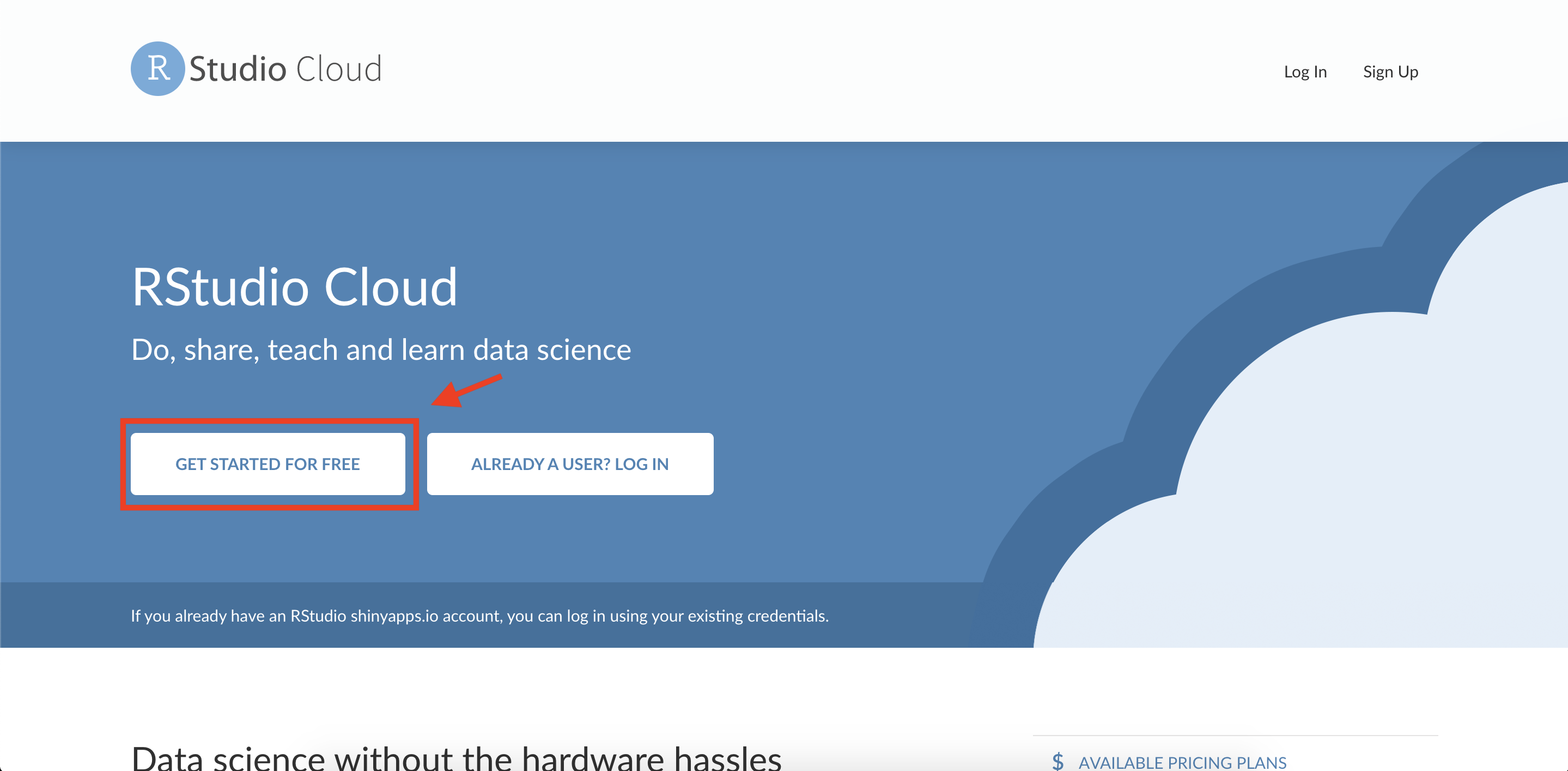2. Click on the **“Sign Up”** button.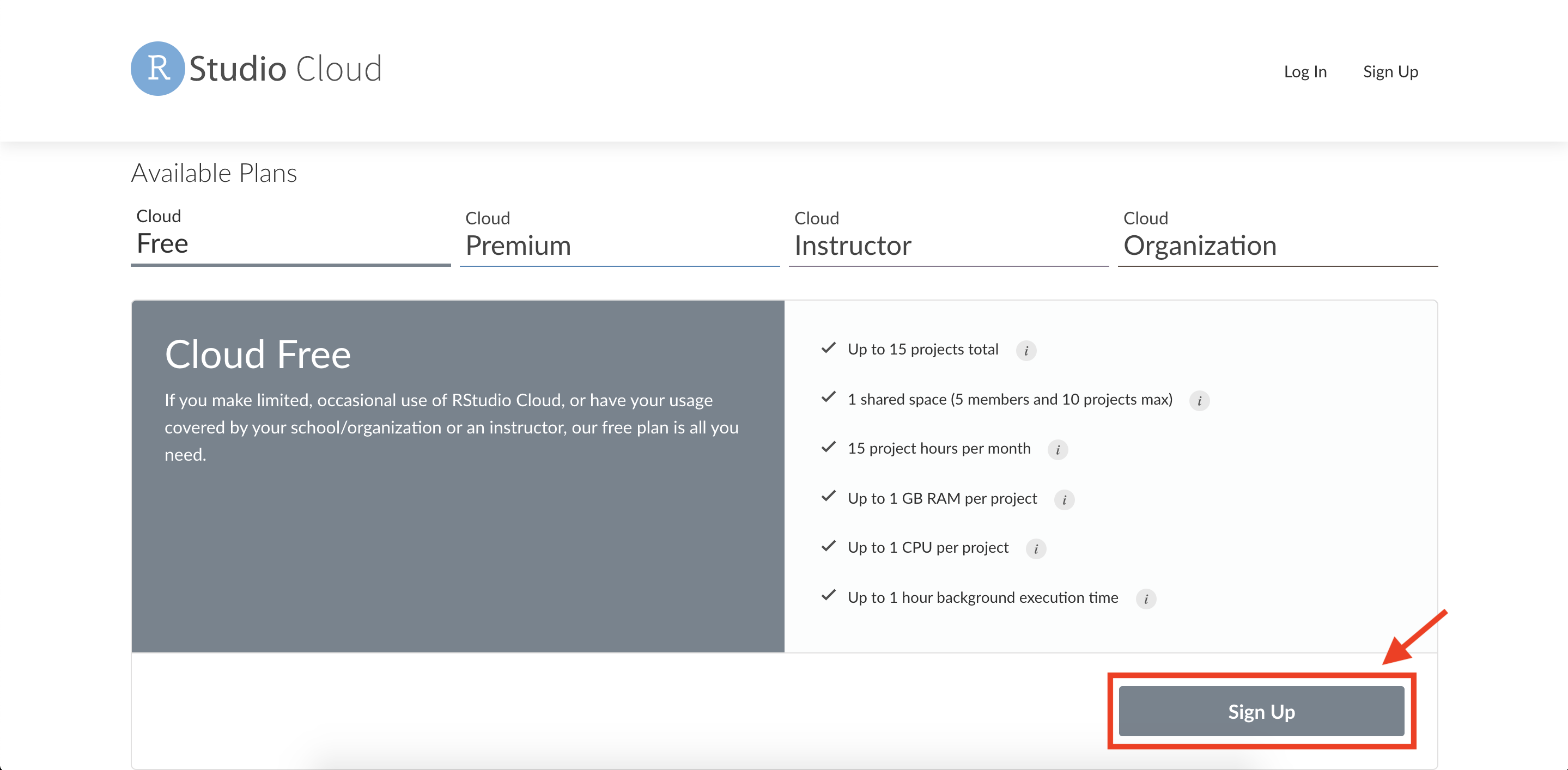3. You will be presented with options to sign up. You can sign up using a Google account, GitHub account, or an email address. Choose whichever method you prefer and complete any required registration steps (such as verifying your email).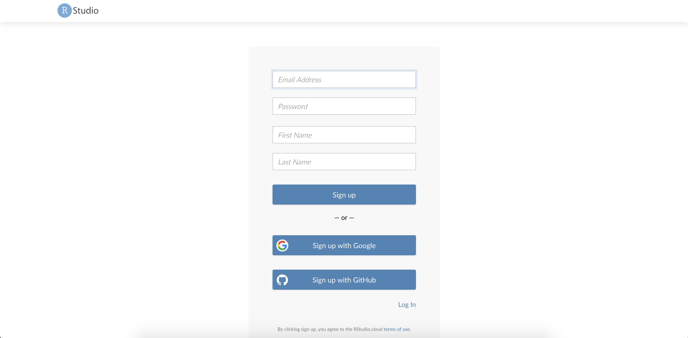4. **Create a New Project:** Once logged in to RStudio Cloud, you will see a dashboard. Click on the **“New Project”** button to create a new RStudio project space.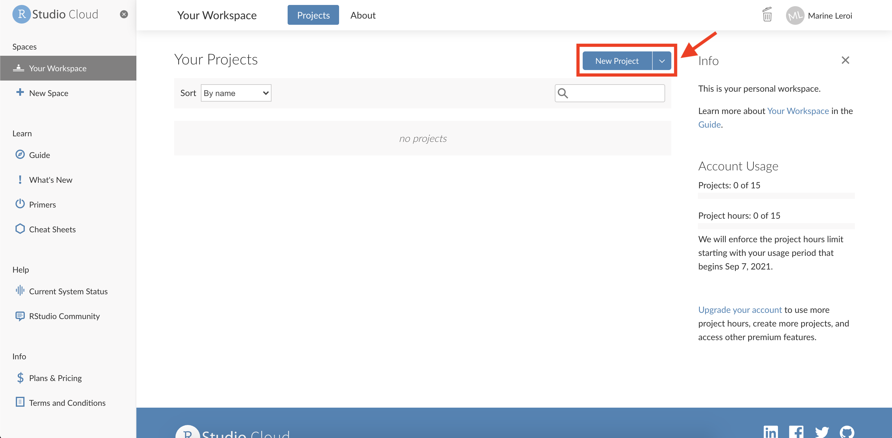5. After a moment, you should see a screen that allows you to configure the new project. You can generally accept the default settings here. The project will be provisioned (this may take a minute as a container with RStudio is started for you).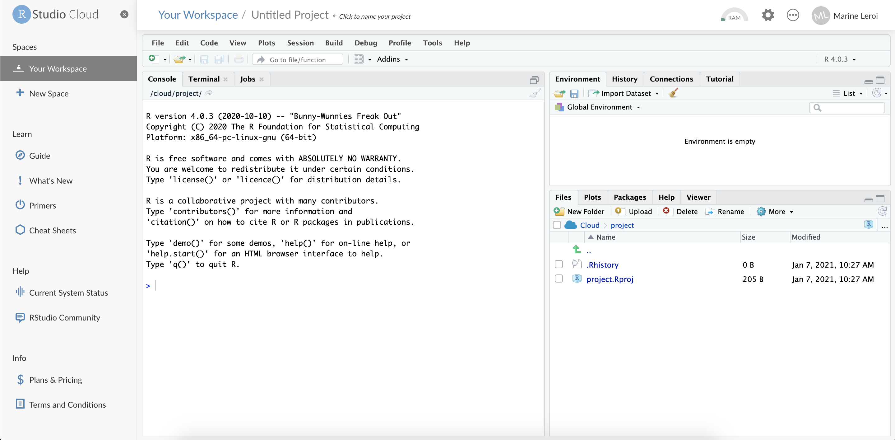6. **Create a new R Markdown file:** Within your new RStudio Cloud project, you’ll be presented with the RStudio IDE interface (which we will describe in detail shortly). To start writing a report, create an R Markdown file. Click on the green **“+”** button at the top-left of the interface (this button creates a new file), and from the dropdown choose **“R Markdown…”**.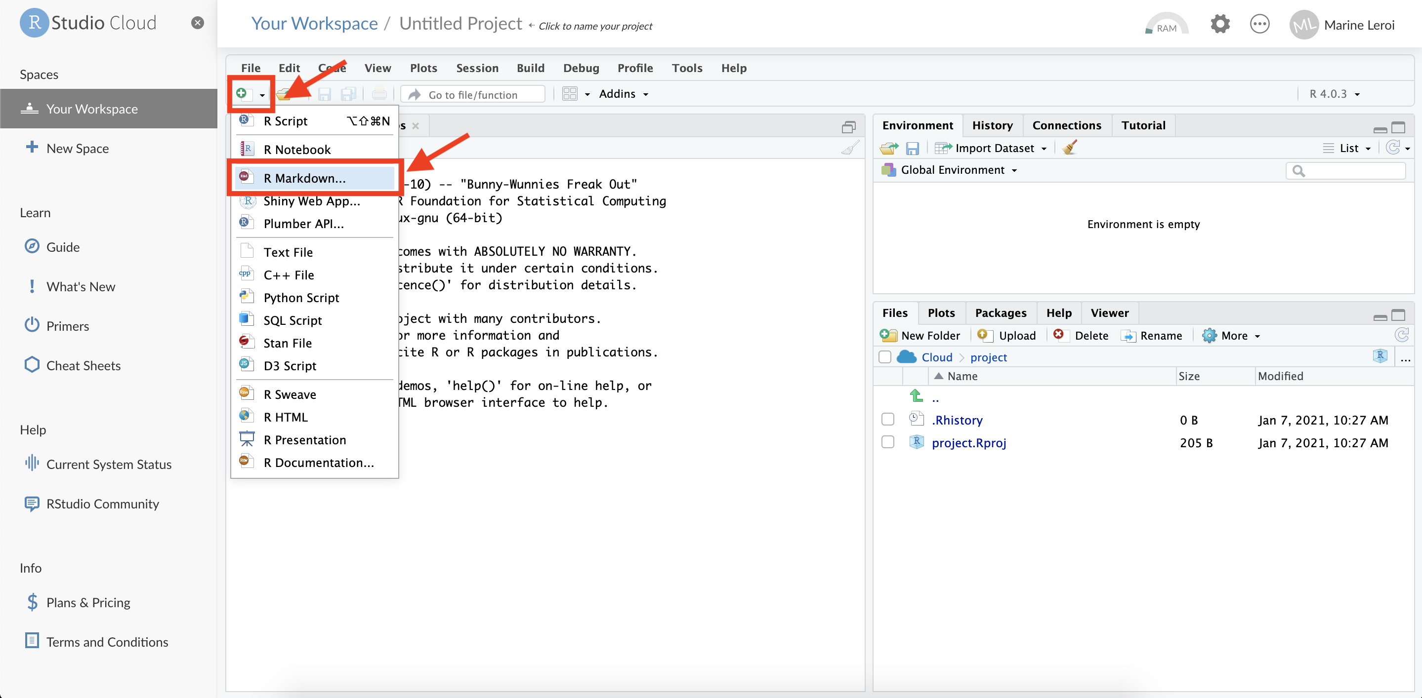7. A dialog window may appear asking if you want to install necessary packages for R Markdown (if this is your first time using it on the project). Click **“Yes”** to install any required packages.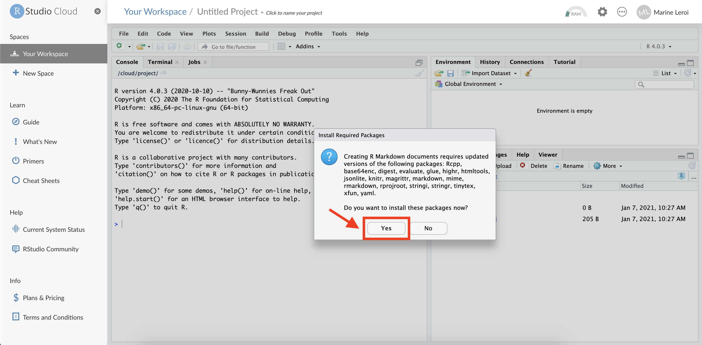8. After a brief pause (while the system installs packages), another dialog window will appear titled **“New R Markdown”**. Here you can set a title and author for your new document. For now, you can leave the defaults or enter a sample title (e.g., “My First Report”) and your name as the author. Ensure the default output format is **HTML**. Then click **“OK”**.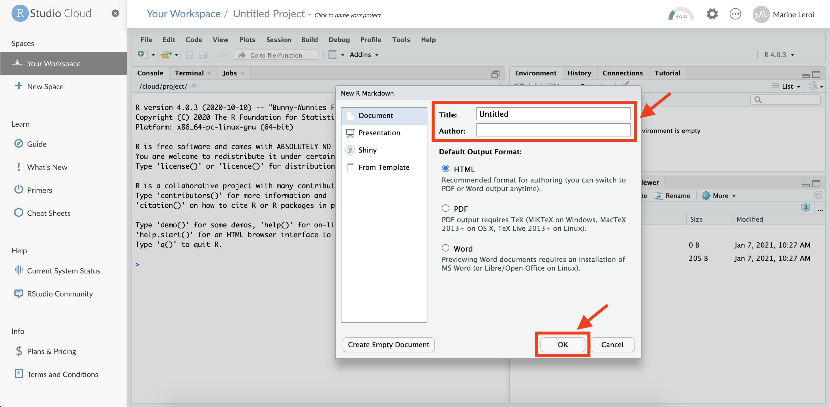9. RStudio will now open a new file tab in the top-left panel with some example content (this is a template R Markdown document). Before we proceed, **save** this file to your project. Click the **floppy disk** icon (💾) or press `Ctrl+S` (Windows/Linux) or `Cmd+S` (Mac).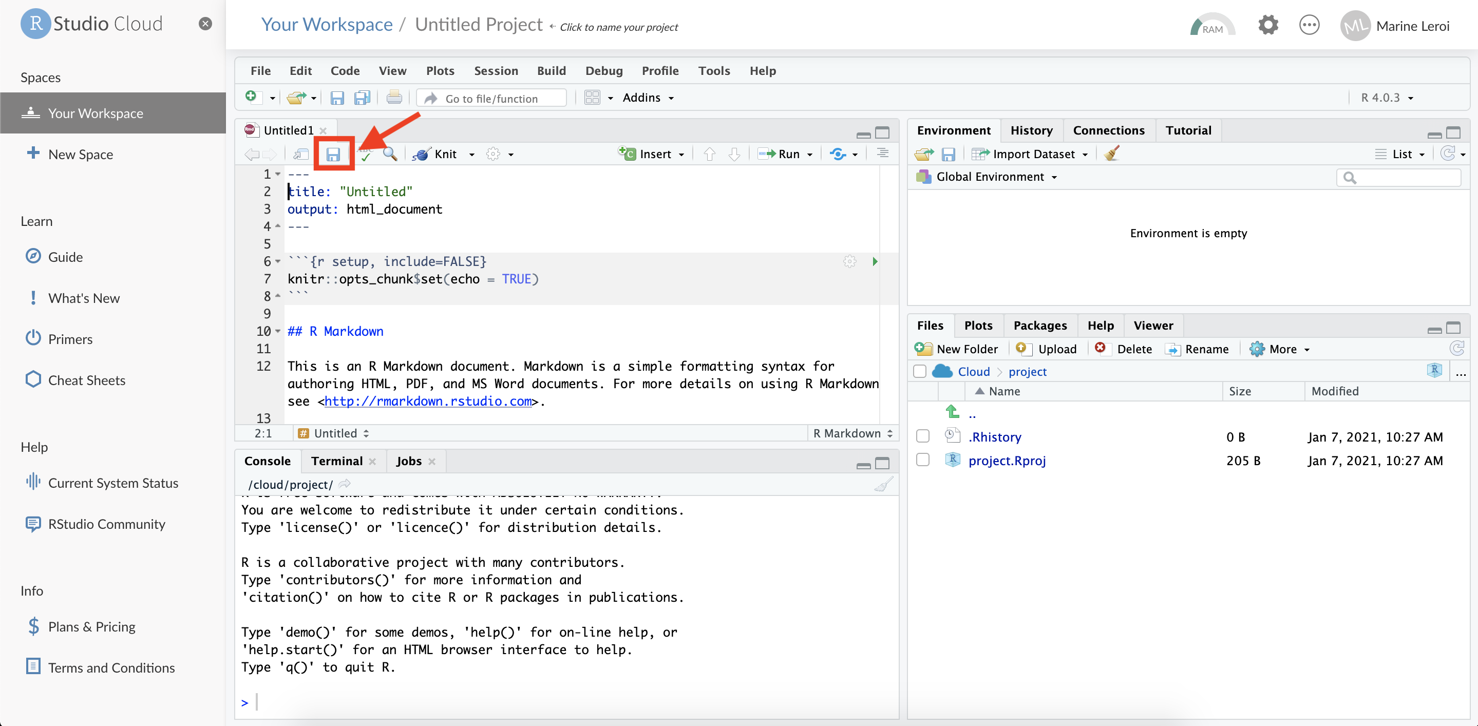10. When prompted, give the file a name (for example, “`first_document.Rmd`”) and confirm the save. Use a name without spaces or special characters (R Markdown files should have the extension `.Rmd`).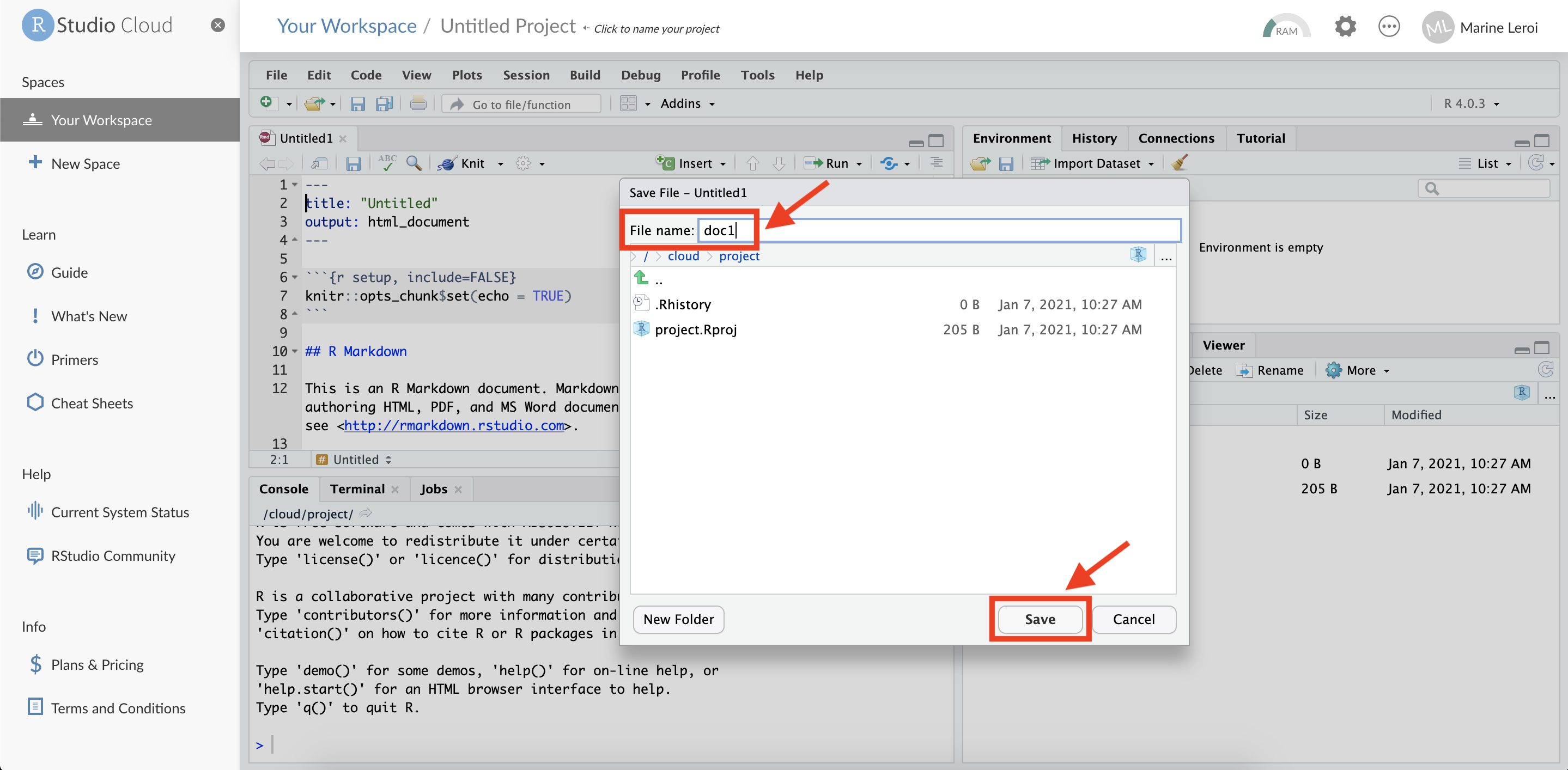11. The new `.Rmd` file will now appear in the **Files** pane (usually the bottom right panel in RStudio). You have successfully created and saved an R Markdown document in your RStudio Cloud project.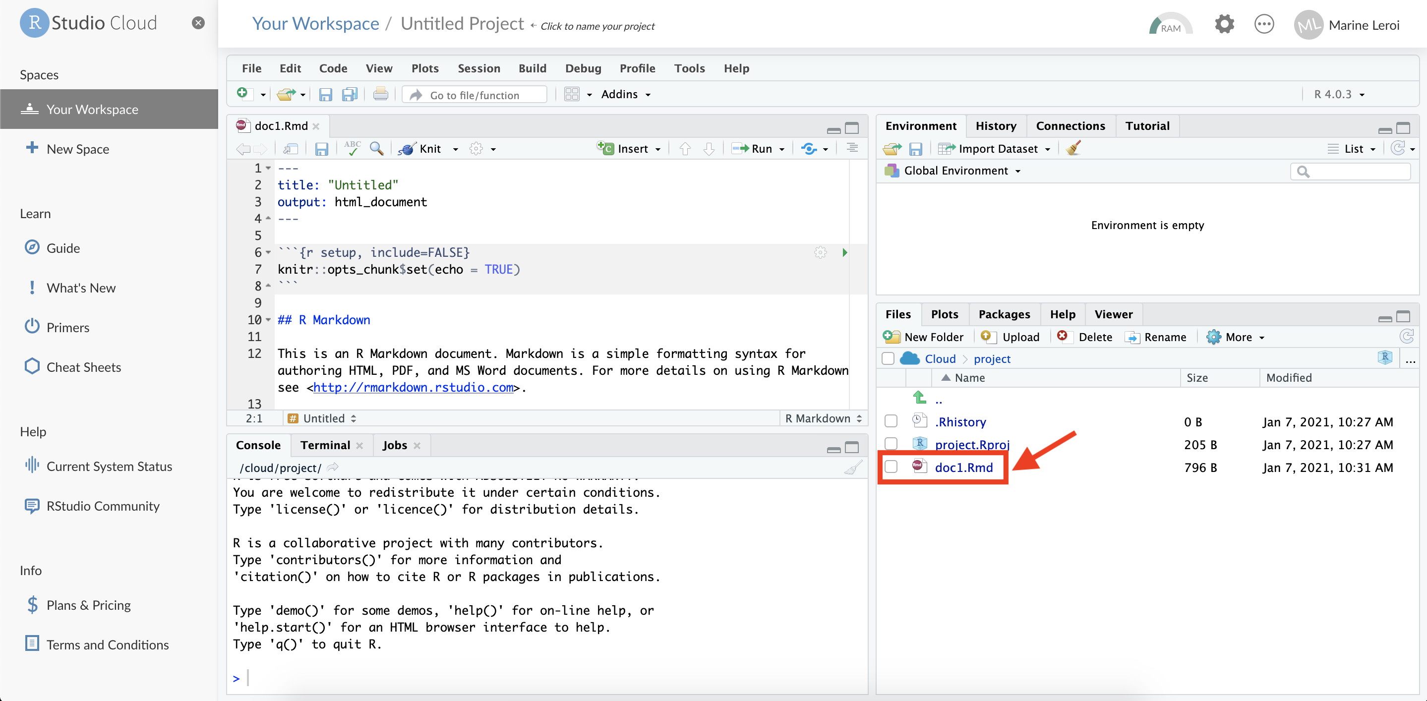At this point, you have an RStudio Cloud account and a project with a simple R Markdown file ready to go. Next, we will take a closer look at the RStudio IDE interface and learn what each part of the screen is for.### Understanding the RStudio InterfaceWhen you open a project in RStudio (whether via RStudio Cloud or the desktop version), the interface is typically divided into **four panels** plus a menu toolbar. Each panel has a specific purpose and knowing what each one does will make you comfortable navigating RStudio as you develop your report.Think of RStudio as analogous to a suite like Microsoft Office, but all integrated into one window. In one part of the screen you might be writing text (like in Word), in another you might be viewing data (like in Excel), and in another you could be typing commands (like a terminal). The difference is that in RStudio these components talk to each other fluidly. For instance, you can run a snippet of code and immediately see the result (a table or a chart) in another panel. Moreover, every time you re-run or *compile* your R Markdown document, you regenerate the analysis with the latest data and code, ensuring your report is always up-to-date.Let’s break down the components of the RStudio interface (assuming the default layout):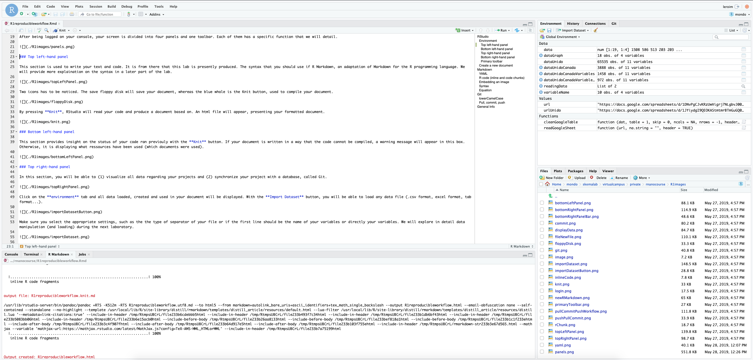{width=600}#### Top Left Panel: Source EditorThe **top left panel** is the **Source Editor**. This is where you write your scripts and documents. In our case, this is where you will write your R Markdown document (with both text and code). You can think of this area as your text editor or word processor that has programming superpowers. For example, the content of this book was written in the R Markdown source editor panel of RStudio.In the editor, you can have multiple tabs open (for multiple files). By default, when we created the new R Markdown file, it opened in a tab here. The content is color-coded for easier reading (for instance, R code might be colored differently than plain text).At the top of this panel, there are a few important buttons: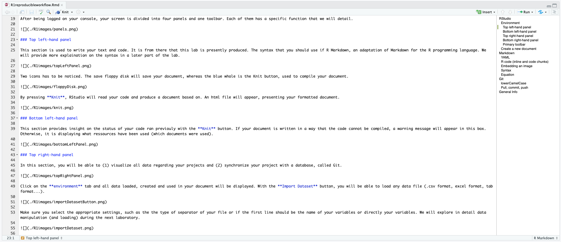{width=600}* The **Save** button (floppy disk icon) saves the current file. Remember to save frequently, especially before trying to run or knit your document.* The **Knit** button (blue icon with a ball of yarn or a circle – it might look like a ball of yarn or a cogwheel depending on your RStudio version) is used to compile your R Markdown document. We often call this “knitting” the document. Pressing **Knit** will tell RStudio to execute all the code in your R Markdown file and produce a formatted output document (by default, an HTML file).{width=600}When you click **Knit**, RStudio will ask you to save the file (if you haven’t already) and then it will run through the document. If all goes well, a preview of your compiled document will appear (often in a pop-up window or in a viewer panel). For an HTML output, RStudio will either show it in its Viewer or open it in your web browser. The compiled document will include all your text, as well as the results of any code (e.g., charts, tables) inserted in the appropriate places.{width=600}Another useful button in the editor toolbar is the **Document Outline** (it looks like a split rectangle or a bullet list icon). Clicking this toggles an outline view of your document (usually appearing in a pane on the left of the editor). This outline is basically a table of contents for your document, listing all the headings and subheadings. This is very handy for navigation as your documents grow longer – you can click on a section title in the outline to jump directly to that part of the document in the editor.{width=600}#### Bottom Left Panel: Console and TerminalThe **bottom left panel** is primarily the **Console**. This is where R commands are executed and results printed. When you click Knit to compile your document, you will see RStudio working through each step in the Console, and any messages, output, or errors will appear here. You can also type commands directly into the console prompt `>` to execute R (or Python, etc., if configured) commands interactively.In the context of knitting an R Markdown document, the console will show you progress and any errors/warnings. For example, if your code has a mistake that causes the document to fail to compile, a red error message will appear in this panel, helping you diagnose the problem. If the document compiles successfully, the console will list the files that were created (for instance, it might say something like “Output created: first_document.html”).The bottom left panel may have multiple tabs aside from the Console. By default, you might also see a **Terminal** tab (which gives you access to a shell command line, if needed) and a **Jobs** tab (for background tasks). For most of our needs, you will be looking at the Console tab in this panel.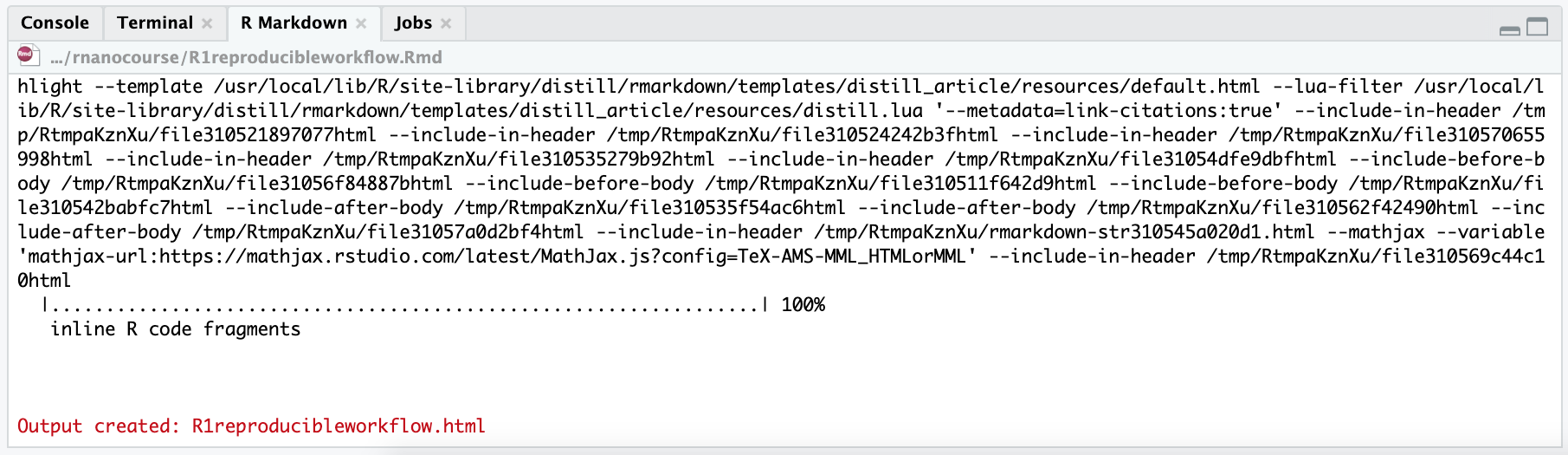{width=600}#### Top Right Panel: Environment and GitThe **top right panel** serves a couple of purposes, primarily data and variable management, and version control. By default, it opens to the **Environment** tab.* **Environment Tab:** This tab lists all the R objects (data frames, variables, functions, etc.) that are currently loaded in your R session. When you load a dataset or create a new variable in your code, you will see it show up here. It’s like your workspace browser. This gives you a quick way to inspect what data you have in memory. For example, if you read a CSV file into a data frame called `salesData`, once that code runs, you’ll see an entry for `salesData` in the Environment tab along with some details like its type and dimensions. You can click on a data frame in the environment to open it in a spreadsheet-like view for a quick look at the data.The Environment tab also has an **Import Dataset** button. This provides a GUI wizard to load data (from text files, Excel sheets, etc.) into R without writing code manually. Clicking this will help you browse for a file and set options (like whether the first row is a header, what the field separator is, etc.) and then import it, generating the corresponding R code for you. While we will teach you how to read data with code (which is more reproducible), this tool can be convenient for quick tasks or for beginners.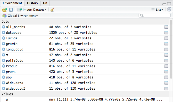{width=600}If you click **Import Dataset**, a dialog will appear where you can select the file and adjust settings. For example, you might choose a CSV file, specify that it’s comma-separated, and indicate that the first row contains column names. RStudio will then read the data and show you a preview. When you confirm, it will load the data into your environment (and you’ll see the data frame listed in the Environment tab).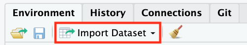{width=300}Make sure to choose the appropriate settings when importing data: the delimiter (comma, semicolon, tab, etc.), whether the first row is a header (variable names) or actual data, how decimal points are represented, etc. Getting these right ensures your data is read correctly. (We will explore data importing and wrangling in detail in later chapters.)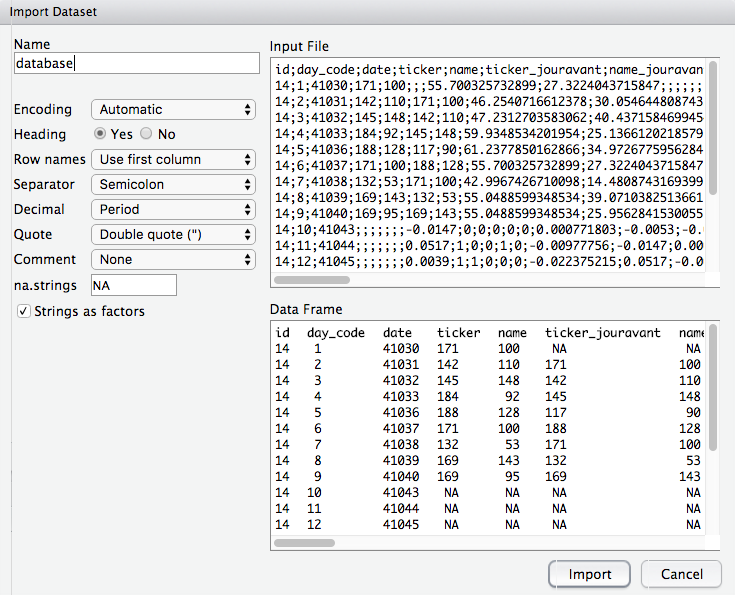{width=600}After importing, if you click on the name of the dataset in the Environment tab, RStudio will open a viewer (usually in the top left panel) showing the first portion (up to 1,000 rows) of the data in a spreadsheet-like format.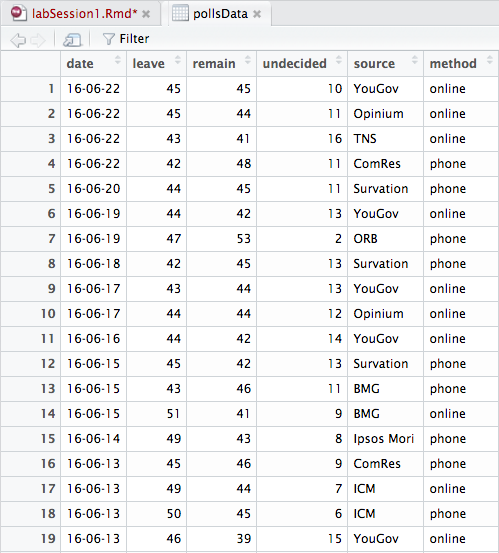{width=600}* **Git Tab:** Next to the Environment tab, you may see a **Git** tab (this will appear if your project is initialized as a Git repository; we will do this soon when we discuss Git). The Git tab will show version control information: which files have been modified, which are staged to commit, etc. From this tab, you can perform Git operations like commit, push, and pull through the RStudio interface. We will cover the specifics in the Git section of this chapter. For now, just note that this is where Git-related info lives in the RStudio interface.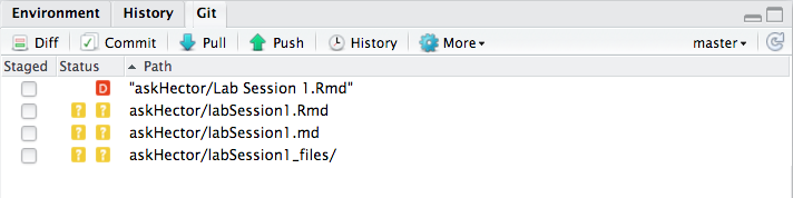{width=600}There may also be a **History** tab in this panel, which logs the commands you have executed in the console.#### Bottom Right Panel: Files, Plots, Packages, Help, and ViewerFinally, the **bottom right panel** is a multipurpose area. By default, it opens to the **Files** tab, which shows the files and folders in your project’s working directory (essentially a file browser, similar to Finder on Mac or Explorer on Windows, but limited to your RStudio project directory).* **Files Tab:** This is where you can see all files associated with your project. You can navigate through sub-folders, and use the buttons provided to manage files. For instance, you can create a New Folder, upload or export files, or delete files. If you select a file, you can use the **More** button (with a gear icon) for additional options like renaming or moving it. One important option here is **“Set As Working Directory”** which tells R (and RStudio) to treat that folder as the base location for relative file paths. By default, when you open an RStudio project, the working directory is set to the project directory, so you usually won’t need to change it. (In our image examples, you might see a working directory path like `askHector`, which was an example project name – the notation `./` in front of paths indicates the current working directory.)When working with R Markdown, it’s good practice to keep your data and images within your project and refer to them with relative paths (like `./data/mydata.csv` or `./images/plot1.png`). The Files tab helps you figure out those paths and manage your project’s content.For example, if you have a subfolder called `images` and inside it an image `diagram.png`, the relative path might be `./images/diagram.png`. We use this path when embedding images in our R Markdown to tell RStudio where to find the file.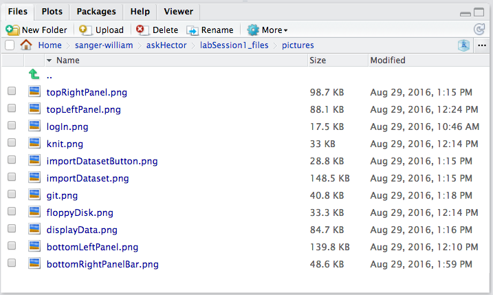{width=600}* **Plots Tab:** Whenever you generate a plot in R (for instance, by calling a plotting function in the console or in a code chunk and running it), it will appear under the **Plots** tab in this panel. You can navigate through previous plots using arrows, zoom into a plot, or export it (save as an image or PDF) from this tab.* **Packages Tab:** This shows a list of R packages installed in your environment, with checkmarks for those that are currently loaded. You can install new packages or update packages using the buttons here, but often it’s just as easy to use `install.packages("packagename")` in the console. Still, the Packages tab provides a quick way to attach a package (by checking its box, which runs `library(packagename)` for you) or see what version is installed.* **Help Tab:** If you use R’s help system (for example, `?mean` or `help(mean)` in the console to get documentation on the `mean` function), the documentation will appear in the Help tab. It’s essentially a built-in web browser for R’s help files and any other documentation you open.* **Viewer Tab:** RStudio has an internal viewer for web content. When you create interactive plots (with packages like `plotly` or `leaflet`) or if you preview an HTML widget or a Shiny app, it might appear in the Viewer tab. Also, when you knit an R Markdown to HTML, by default RStudio might show it in this Viewer instead of your external web browser.Think of the bottom right panel as your miscellaneous toolbox: file manager, plot viewer, package manager, help browser, etc., all in one.As an example of using the Files tab, consider the path example from above. We mentioned an image with path **`./R1images/bottomRightPanel.png`** in a description. That path indicates there is a folder named **R1images** in the current project, and inside it a file `bottomRightPanel.png`. Knowing how to read and use such paths is important when you link resources in your R Markdown (like including images or data files). The Files pane can help you verify those file names and paths.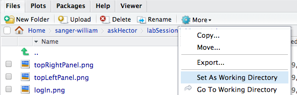{width=600}In the Files pane, you have controls to manipulate files:* **New Folder** button: create a new directory in your project.* **Upload** (in RStudio Cloud or if enabled): bring files from your local system into the project.* **More** (gear icon): contains options to Rename, Delete, or Export (download) selected files, and as mentioned, **Set As Working Directory** which changes R’s reference point for relative paths.Generally, you won’t need to set the working directory manually if you stick to using RStudio Projects, because the project’s main directory is automatically the working directory.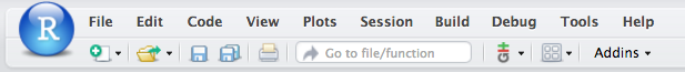{width=600}#### Primary Toolbar and MenusAt the very top of RStudio (above all panels) is the primary menu bar and toolbar. This includes menus like **File, Edit, Code, View, Plots, Session, Build, Git, Tools, Help** (these may vary slightly if using RStudio Desktop vs Cloud). Many of the functions accessible through buttons in the panels are also available via these menus.Key items include:* **File menu:** Create new files, open recent projects, save files, etc.* **Edit menu:** Text editing functions (undo, copy, paste, find/replace, etc.).* **Code menu:** Useful code editing shortcuts (comment/uncomment lines, reindent code, etc.).* **Run menu (or on toolbar):** Buttons to run code from the source editor (like running the current line or selected code, which sends it to the Console).* **View:** Options to zoom or rearrange panels.* **Session:** Controls for your R session (restart R, interrupt running code, set working directory, etc.).* **Git (if a Git repo):** Quick access to version control operations.* **Tools:** Global options, addins, managing packages, etc.* **Help:** Access documentation and diagnostics.In addition to menus, the toolbar typically has icons for common actions (New file, Open file, Save, Knit, Run, etc.). We will explore certain toolbar features (like **Addins**) later in this chapter when we discuss the citr add-in for citations.**To go further:** If you want to set up R and RStudio on your own computer (instead of or in addition to using RStudio Cloud), there is a tutorial available that walks through installing R, RStudio, and necessary packages. You can refer to [this guide](https://warin.ca/posts/rcourse-rnanocourse0/) for detailed steps on local installation and configuration.**TL;DR** – *RStudio Interface Overview*:* **IDE (Integrated Development Environment):** A software application (like RStudio) that provides comprehensive facilities to programmers for software development, combining a source code editor, build automation tools, and more, in one GUI.* **RStudio environment is split into four main panels:** * **Top Left (Source Editor):** Where you write your text and code (R scripts, R Markdown files, etc.). This is your main coding area with a text editor and action buttons like Save and Knit. * **Bottom Left (Console/Terminal):** Where code runs and output or error messages appear. You can also type commands here directly. It shows the log and progress when knitting documents. * **Top Right (Environment/History/Git):** Shows your data and variables in the Environment tab. Also includes the Git tab for version control (when using Git) and can show command history. * **Bottom Right (Files/Plots/Packages/Help/Viewer):** A multipurpose area for browsing project files, viewing plots, managing packages, reading help files, and previewing web content or reports.By understanding what each panel does, you can efficiently navigate RStudio and make the most of its features while developing your data analysis projects.Thanks! I’ll retain the R Markdown material as-is, then add a new section introducing Quarto (.qmd), including its differences from R Markdown, advantages, and the ability to use other languages like Python or Julia in code chunks. I’ll let you know as soon as that section is ready.## Writing Documents with R Markdown (and Quarto)Now that you have set up the RStudio environment, let’s focus on creating content using **R Markdown**. (We will also introduce **Quarto**, a newer system similar to R Markdown, later in this section.) R Markdown is one of the two main tools we will use throughout this book (the other being R itself). It allows you to combine regular text (formatted in a simple, readable way) with chunks of R code. When you *knit* an R Markdown document, the code is executed and its output is embedded in the final document, which can be rendered to various formats like HTML, PDF, Word, or even presentation slides.Using R Markdown is central to the concept of **reproducible research**: your report is reproducible because anyone with your R Markdown file and data can re-run it to get the same results. If the data are updated or the analysis needs to change, you edit the code in one place (the R Markdown file) and knit again to produce an updated report. This is much more efficient and less error-prone than manually updating numbers or plots in a Word document.In this section, we will create a simple R Markdown document and learn the basics of the Markdown syntax and structure. *(If you followed the steps in the RStudio Cloud setup, you have already created an R Markdown file with a sample template. We will use that as a starting point. If not, here is how you can create a new R Markdown document in any RStudio session.)*### Creating a New R Markdown DocumentTo create a new R Markdown document in RStudio, use the menu: **File > New File > R Markdown...**. This will open a dialog for specifying the title, author, and output format of your new document.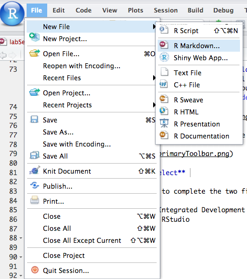{width=600}Choose **Document** (the default) as the type of R Markdown (as opposed to Presentation or other specialized formats) and ensure the default output is HTML. Enter a title and author if you’d like (you can change these later in the document’s YAML header). Then click **OK**.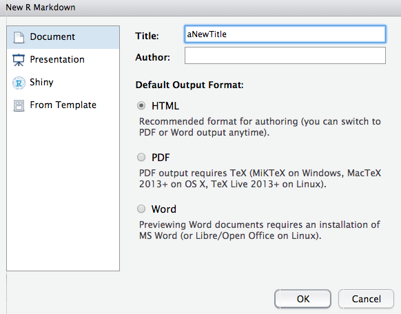{width=600}RStudio will create a new file (with some example content) and open it in the source editor. Don’t forget to **save** this file (with a name ending in `.Rmd`). Once saved, you can proceed to edit the content.At this point, if you have been following along, you should have achieved a couple of things already:* Familiarized yourself with the RStudio IDE layout.* Created (and saved) your first R Markdown document in RStudio.Now we will dive into how to write in R Markdown.### The Structure of an R Markdown DocumentAn R Markdown document has three basic components:1. The **YAML header** at the very top (optional but important for specifying document metadata and output options).2. The **body** of the document, which includes your narrative text mixed with **code chunks** that execute R (or other languages’) code.3. (Possibly) a section for **references** at the end, if you are citing sources (we will cover citations later).Let’s go through these components and some key syntax elements of Markdown.#### YAML HeaderYAML stands for “YAML Ain’t Markup Language” (a recursive acronym) – essentially, it’s a human-readable format for specifying configuration. In an R Markdown file, the YAML header is the section at the very top enclosed by triple dashes `---` at the beginning and end. It provides metadata about the document and instructions for the output format.Here’s an example of a simple YAML header in an R Markdown (.Rmd) file:```yaml---title:"My First Report"author:"Jane Doe"date:"26/06/2025"output: html_document---```This YAML header specifies:* **title:** The title of the document (appears at the top of the report).* **author:** The author name (appears below the title in many formats).* **date:** The date (or any text you want in the date field).* **output:** The output format. Here `html_document` means we want to knit to an HTML file. Other common options include `pdf_document` for PDF output, `word_document` for a Word .docx file, `beamer_presentation` for a PDF slide deck, `ioslides_presentation` for HTML slides, and `github_document` for a Markdown output suitable for GitHub. You can change this depending on what final format you need.You can add many other options in YAML. For example, `toc: true` will include a table of contents, `bibliography: references.bib` can specify a file for references (useful when you need to cite sources), or you can specify visual themes for slides and documents. In our simple documents, we’ll often stick to just the basic fields shown above.The YAML header is incredibly convenient because it lets you switch the entire output format or other settings without touching the main body of your document. For instance, if you wrote a report and later need it as a presentation, you can change `output: html_document` to `output: ioslides_presentation` (and maybe tweak a few things in the content) and knit again to get slides. The same content can be output in different forms with minimal effort.One thing to note: If you are used to word processors, you might be tempted to adjust the formatting of specific sections manually (like making one heading a different color or a specific line a larger font). In R Markdown (and Quarto), a lot of that fine-grained control is handled by the output format’s template or by using custom CSS/LaTeX templates, rather than in the document content itself. The idea is that you focus on content, and let the template handle the style. This can be a mental adjustment: you give up a bit of *immediate* control over appearance in exchange for consistency and speed. The upside is huge – you won’t spend time tweaking formatting on every update, and your documents will have a professional, consistent style. The downside is you may need to learn a bit about styling (CSS or LaTeX) if you want to customize beyond the provided templates, but for most cases you can find a template or default that looks good.*(If you ever need to highly customize appearance, you can. But as a tip: content is king. It’s often better to use the default styles unless you have a compelling reason – they are usually chosen by experts in design to be clean and readable.)*#### R Code ChunksThe real magic of R Markdown is its ability to run code and insert the results into the final document. This is done with **code chunks**. A code chunk in R Markdown looks like this in the source:<pre>```{r}# This is an R code chunksummary(cars)```</pre>Everything between the ` ```{r} ` and the closing ` ``` ` is interpreted as R code (not as text for the report). When you knit the document, that R code will be executed. Anything the code prints to output (like the summary of a dataset, or a plot) will be captured and inserted into the document at that position.Let’s break down the example chunk above:```{r}summary(cars)```Here, `cars` is a built-in dataset in R (a simple data frame of car speeds and stopping distances). `summary(cars)` will produce summary statistics for each column (min, max, mean, etc.). When you knit the document, those statistics will appear in the output at the position of the chunk.If you have multiple lines of code in one chunk, they will all run in sequence. You can also include comments in your code (lines starting with `#`), which are ignored by R when running. Comments in code chunks will not appear in the output document (they’re not text for the report, just notes to yourself in the source).Another example chunk might be:```{r}# Plot a scatterplot of the cars dataplot(cars)```This chunk, when run, will produce a scatter plot of the `cars` dataset (speed vs stopping distance), and that plot image will be inserted into the document.By default, code chunks will also **echo** the code (show the code itself) in the output document, followed by the results or plot. However, you can control chunk behavior with **chunk options** inside the curly braces `{ }` that start the chunk. For example:* `{r, echo=FALSE}` – runs the code *without* showing the code in the output (only the results will appear).* `{r, include=FALSE}` – runs the code but includes neither the code nor the results in the output (useful if you need to set something up in code that the reader doesn’t need to see).* `{r, eval=FALSE}` – shows the code in the output but does *not* actually execute it (useful for showing code examples without running them).There are many such options (like controlling figure size, whether to cache results for speed, etc.), but we won’t overwhelm you with those now. The default behavior is usually fine for learning purposes.In RStudio’s editor, you can also run individual chunks without knitting the whole document by clicking the little green triangle “play” button that appears to the right of a chunk, or by using the shortcut `Ctrl+Shift+Enter` (Windows) or `Cmd+Shift+Enter` (Mac) when your cursor is inside a chunk. This executes the chunk and shows you the output in the console or plot pane, which is handy for testing and iterative work.#### Inline CodeSometimes you want to embed a single value or a small result directly in your text, rather than showing it as a separate block. For example, you might want to write: “The average speed is 15.4 mph” where that number is calculated from data. Hard-coding such numbers in text is not reproducible (if the data updates, your text would be wrong unless you remember to update it too), but R Markdown allows **inline code** to solve this.Inline R code is written using a single backtick `` ` `` followed by `r` and the code, then another backtick. For example: `` `r mean(cars$speed)` `` in your text will be replaced by the result of the R expression `mean(cars$speed)` when the document is knit.So you could write in your R Markdown file:```markdownThe average speed of the cars dataset is `r mean(cars$speed)` miles per hour.```When you knit, that will become something like:*“The average speed of the cars dataset is 15.4 miles per hour.”* (assuming 15.4 is the actual mean of that dataset).Inline code is extremely useful for embedding statistics or results in your narrative. It ensures consistency between what your analysis calculates and what you describe in the text, because the value is generated dynamically. If your data changes or you do a different analysis, the narrative text will update on the next knit.One thing to note: inline code should be brief. It’s not meant for long computations or producing plots; it’s for a single number or a short piece of text. Also, by default inline results are inserted as plain text (if they’re numeric, they’ll be formatted as numbers). You can control formatting (like number of decimal places) using R functions or formatting options if needed (for example, using the `round()` function inside the inline code to round a number).#### Basic Markdown Syntax for TextNow let’s cover how to format the text itself in your R Markdown document using Markdown syntax. Markdown is designed to be simple and readable as plain text, while allowing for basic formatting. Here are some common elements:* **Headings:** Use the `#` symbol to denote headings. The number of `#` you use indicates the level of the heading. For example: * `# Heading 1` (usually the document title; if you use the YAML title, you typically don’t need to put a level-1 heading in the body). * `## Heading 2` (a major section heading). * `### Heading 3` (a subsection). * You can continue to smaller sub-sections with ####, #####, etc., but rarely do you need more than 3-4 levels in a short report. In the output, these will be formatted with decreasing font sizes or emphasis. They will also be used to build a table of contents if you enabled `toc: true` in the YAML.* **Bold and Italic text:** * To make text **bold**, wrap it in double asterisks, like `**this**`, or in double underscores `__this__`. * To make text *italic*, wrap it in single asterisks `*this*` or single underscores `_this_`. * You can combine for ***bold and italic*** with triple asterisks/underscores, but that’s less common.* **Lists:** * **Unordered lists (bulleted lists):** Start a line with a dash `-` or an asterisk `*`. Indent by 2 spaces (or a tab) to create sub-lists. For example:```markdown - First bullet item - Second bullet item - Sub-item - Sub-item - Third bullet item``` will produce a bulleted list with a sub-list under the second item. * **Ordered lists (numbered lists):** Start lines with `1.`, `2.`, etc. The numbers will automatically display in order when rendered (you can actually just put `1.` for each and Markdown will number them correctly). ```markdown 1. Step one 2. Step two 3. Step three ``` will produce an ordered list of steps. * You can mix lists with paragraphs or sublists, but be careful with indentation so that Markdown knows what is part of a list versus a new paragraph.* **Links:** To insert a hyperlink, use the format `[link text](URL)`. For example: `[RStudio website](https://www.rstudio.com){target="_blank"}` will render as a clickable link: [RStudio website](https://www.rstudio.com). (The `{target="_blank"}` part is optional; it makes the link open in a new tab for HTML output.)* **Images:** In Markdown, images are inserted similar to links but with an exclamation mark prefix. The syntax is ``. You can include alternative text inside the brackets for accessibility (in case the image doesn’t load). For example:```markdown{width=200}``` will include the image at that path, scaled to a width of 200 pixels (the `{width=...}` is a way to suggest a display width; it’s especially useful for LaTeX/PDF output for controlling image size). In our documents, we often provide images with a specific width for consistency. In this chapter, we have an `images` folder in our project, and we reference images by their relative path. This keeps the document self-contained (as long as the images folder accompanies the document).* **Code formatting in text:** If you want to refer to a piece of code or a filename in your narrative (without executing it), you can format it as code by wrapping it in single backticks. For example, “Use the function `mean()` to calculate the average” or “Open the file `analysis.Rmd` for editing.” This will display the text in a monospaced font and distinguish it as code.* **Blockquotes:** If you want to quote a passage or provide a highlighted note, start the line with `>`. For example:```markdown> Data science is the art of turning data into actions.``` will appear as an indented block quote. (We won’t use blockquotes often for our purposes, but it’s good to know.)These are the most frequently used Markdown elements for basic writing. There are others (like tables, which we’ll see later when discussing references and citations, or horizontal rules using `---` or `***`), but the above covers the essentials. You can always refer to the RStudio Markdown cheatsheet for a quick reference on syntax ([**R Markdown Cheat Sheet (PDF)**](https://www.rstudio.com/wp-content/uploads/2015/02/rmarkdown-cheatsheet.pdf){target="_blank"}).#### Adding Mathematical NotationIf you need to include mathematical equations or symbols, R Markdown (via Pandoc’s Markdown) allows you to use LaTeX math notation:* For **inline math**, wrap the LaTeX in single dollar signs. Example: ```markdown The formula for the line is $y = \alpha_0 + \alpha_1 x_1 + \alpha_2 x_2 + \epsilon$. ``` This will render inline, for example: *The formula for the line is $y = \alpha_0 + \alpha_1 x_1 + \alpha_2 x_2 + \epsilon$.** For **display (centered) equations** that appear on their own line (typically numbered in scholarly writing), use double dollar signs on separate lines:```markdown $$ y_i = \alpha_0 + \alpha_1 x_{i1} + \alpha_2 x_{i2} + \alpha_3 x_{i3} + \epsilon_i $$``` This will display the equation centered on its own line: $y_i = \alpha_0 + \alpha_1 x_{i1} + \alpha_2 x_{i2} + \alpha_3 x_{i3} + \epsilon_i$You can include Greek letters (e.g., `\alpha` for α), subscripts with `_` (e.g., `x_{i1}` for $x_{i1}$), superscripts with `^` (e.g., `x^2` for $x^2$), fractions with `\frac{a}{b}`, summation symbols `\sum`, and so on. Essentially, anything you could write in LaTeX math mode can be done in R Markdown. This is extremely powerful for reports that include statistical or mathematical formulas.#### Knitting the DocumentOnce you have some content in your R Markdown file – a combination of text, code chunks, etc. – you can generate the output by clicking the **Knit** button in RStudio. It’s the button with a ball of yarn icon and a needle, at the top of the source pane. If you’re not using RStudio, you can also knit by calling a function in R (e.g., `rmarkdown::render("your_file.Rmd")`), but in RStudio the button is easiest.When you click **Knit**, RStudio will run through the document, executing each code chunk in a clean R session, capturing the output and plots, and then assembling everything into the final document (HTML, PDF, etc., depending on your YAML). If there are errors (for example, a chunk of R code has a mistake), the knitting process will stop and you’ll see an error message in the R console. You would then fix the issue and knit again. If all goes well, you’ll get an output document in your chosen format.For example, if you knit the default sample R Markdown that RStudio created when you made a new file, you’ll get an HTML page with a title, some introductory text, a plot of the `pressure` dataset, and a few other examples. RStudio will likely open this in its Viewer pane (or you can open the HTML file in a web browser).Every time you knit, you’re running a fresh execution of the document. That means it’s **reproducible** – the output document doesn’t rely on anything you did before by hand (you’re not copy-pasting results; the code in the document always generates the results from scratch). It also means that if you change the data or update a parameter in your analysis, those changes will be reflected the next time you knit. This ensures your report is always in sync with your latest analysis or data.By this point, you should be comfortable creating an R Markdown file, writing basic content with Markdown formatting, and including R code to perform computations or generate plots. You should also be able to click Knit and produce a nicely formatted output document that combines text and code results.**Reproducible Research Note:** We emphasize reproducibility because it saves time and avoids errors. For instance, imagine using R Markdown for a business report: next month you get new data, so you update the data file and re-knit the report. All the tables and figures update automatically based on the new data. Contrast this with a manual process (like updating numbers in Excel and copying them into Word) – that approach is tedious and prone to mistakes. Embracing tools like R Markdown means your work is not only more efficient for yourself, but also easier to hand off to someone else or to revisit after time, since everything needed to regenerate the results is in one place (the script and the data).As a real-world example of reproducible research and transparency, consider an initiative in academia: many journals encourage or require authors to publish replication materials. For example, there is a repository of academic articles in economics where each paper’s data and code are made available so others can reproduce the findings. You can explore one such repository here: [**Economic Articles – Reproducible Research**](https://ejd.econ.mathematik.uni-ulm.de/){target="_blank"}. This site lists economics papers that come with code and data, allowing anyone to rerun the analysis. It’s a good reminder of the growing expectation in many fields that results should be reproducible.**TL;DR – *Key R Markdown Elements:**** YAML header at the top (between `---` lines) defines document title, author, date, and output format (among other options).* Write narrative text in Markdown: use `#` for headings, `**bold**` or `*italic*` for emphasis, `-` for bullet lists, `1.` for numbered lists, etc.* Include R code in **code chunks** like:<pre>```{r}summary(cars)```</pre> This will run the code and include its output (or plot) in the document.* Include **inline R code** with `` `r` `` to insert computed values into your text.* Embed an image with Markdown syntax, e.g. `` (optionally with size attributes like `{width=400}`).* Write equations with LaTeX syntax: `$E = mc^2$` for inline or `$$E = mc^2$$` for a standalone formula.* Click **Knit** to compile the document and see the output. If using a different environment, run the render function to produce the output file.Some R functions we used in the examples above:* `summary(object)` – produces summary statistics of a dataset or R object.* `plot(object)` – produces a plot (the output depends on the type of object; for a data frame like `cars`, it will make a quick scatter plot).* `mean(vector)` – calculates the mean of a numeric vector.### Quarto (.qmd): A Modern Alternative to R MarkdownBy the way, there’s a newer tool called **Quarto** that you might hear about. Quarto (with file extension `.qmd`) is essentially the next generation of R Markdown, introduced by Posit (formerly RStudio) in 2022. It extends the ideas of R Markdown to be **multi-language and multi-engine**. In practical terms, a Quarto document looks and feels very much like an R Markdown document: you write Markdown text, you include code chunks, and you render the document to formats like HTML, PDF, Word, slides, etc. The big difference is that Quarto isn’t limited to R – it allows you to use Python, Julia, JavaScript, and other languages in your code chunks, in addition to (or instead of) R.If you are only using R, Quarto will behave almost identically to R Markdown for your purposes. In fact, Quarto can render most existing `.Rmd` files without modification. But Quarto provides a unified framework for doing more, and it’s likely to be the focus of new features going forward. Here, we’ll give a brief overview of Quarto and how it compares, so you’re aware of it.**Creating a New Quarto Document:** To create a Quarto document in RStudio (version 2022.07 or later), you can use the menu **File > New File > Quarto Document**. This is analogous to creating an R Markdown file. When you do this, you’ll get a new file with extension `.qmd`. The RStudio IDE will recognize it as a Quarto file. The sample content of a new Quarto document is very similar to the R Markdown template, just with slight differences in the YAML and perhaps an example of a Python chunk. Don’t forget to **save** the file (with a `.qmd` extension).The RStudio IDE shows a **Render** button (often a blue circle icon with a white “Q”) when you have a Quarto document open. This replaces the Knit button for `.qmd` files. Clicking **Render** will execute the Quarto workflow (which, behind the scenes, runs the code and uses Pandoc to create the output). The experience of writing and rendering is otherwise quite similar to R Markdown. You can also render Quarto documents from the command line using `quarto render mydocument.qmd` or from R by using the Quarto R package (`quarto::quarto_render("mydocument.qmd")`), but using the RStudio button is easiest when you’re working interactively.**Structure of a Quarto Document:** A `.qmd` file also has three main parts, much like R Markdown:1. A YAML header at the top (between `---` lines) for title, author, output format, etc.2. The body of the document with Markdown text and code chunks.3. An optional references/bibliography section at the end (if you need to cite sources).Everything you learned about writing Markdown text (headings, lists, bold/italic, links, images, etc.) and including mathematical notation applies equally to Quarto. The Markdown syntax is the same. The idea of **code chunks** is also the same, but with Quarto you are not restricted to R for those chunks.**YAML in Quarto:** The YAML fields in a Quarto document are largely the same, but the **output format** is specified a bit differently. Instead of `output: html_document` (which was specific to the R Markdown system), Quarto uses `format` to specify output. For example, a simple Quarto YAML might be:```yaml---title:"My First Report (Quarto)"author:"Jane Doe"date:"26/06/2025"format: html---```This tells Quarto to produce an HTML document. If you wanted a PDF, you would use `format: pdf`. For a Word document, `format: docx`. Quarto has short, intuitive names for formats (it consolidates what was a variety of output functions in R Markdown into a single system). You can even list multiple formats if you want to render to, say, HTML *and* PDF at the same time (Quarto can target multiple outputs in one render, using a list under `format` field). For example:```yaml---title:"Report"format:html: defaultpdf: default---```would produce both HTML and PDF outputs with one command. But for now, you can stick to a single format like HTML.All the other YAML options (title, author, date, toc, etc.) work similarly in Quarto. In fact, you’ll often find that you can copy an R Markdown YAML header into a Quarto doc and just adjust the `output`/`format` field and it works.**Code Chunks in Quarto:** Quarto’s code chunks are very flexible. You still delineate a code chunk with triple backticks and curly braces, but instead of always `{r}`, you indicate the language. For example:* An R chunk: ` ```{r} ` (just like before).* A Python chunk: ` ```{python} `.* A Julia chunk: ` ```{julia} `.* Even an Observable JavaScript chunk: ` ```{ojs} ` (for advanced interactive JS, if needed).Within one Quarto document, you can have some chunks in R and others in Python (or other languages). Quarto will automatically use the right engine to run each chunk. For R, it uses **knitr** (just as R Markdown does). For Python, Quarto can either use an embedded Python session or Jupyter behind the scenes. The result is that you can mix R and Python in one report seamlessly.For example, here’s a tiny Quarto document body with mixed languages:<pre>Some analysis in R:```{r}x <-1:5mean(x)```And now a quick check in Python:```{python}numbers = [1, 2, 3, 4, 5]sum(numbers) /len(numbers)```</pre>When you render this Quarto document, the first chunk will execute in R (calculating the mean of 1 through 5, which is 3), and the second chunk will execute in Python (doing the same computation in Python). The results from each chunk will be inserted in the final document. In this case, both would output the value 3 (plus any printed output if present).Just like in R Markdown, you can include **comments** in your code with `#` (for both R and Python), and you can control whether code is shown or hidden, executed or not, using chunk options. Quarto actually introduces a slightly different way to specify chunk options: you can write them as lines starting with `#|` inside the chunk (this is a YAML-like syntax for options). For example:<pre>```{r}#| echo: false#| fig-width: 6plot(cars)```</pre>In this Quarto R chunk, we set `echo: false` (so the R code won’t be shown) and `fig-width: 6` (inches) for the resulting plot. This new `#|` syntax is optional; Quarto will also understand the old way (`{r, echo=FALSE}`) for compatibility. Use whichever style you prefer. The key point is that chunk options and their effects (hiding code, figure size, etc.) behave the same in Quarto as they do in R Markdown.**Inline code** in Quarto is also supported and works the same way: use `` `r 2+2` `` or even `` `python 2+2` `` inside your text to evaluate expressions. By default, Quarto assumes an unlabeled inline code chunk is in R (since it originated in R Markdown), so to be safe when using other languages inline, you prefix the language like `` `python` ``. In practice, most people use inline code for simple numerical results and typically with R, but it’s good to know you have options.**Rendering a Quarto document:** As mentioned, if you’re using RStudio, click the **Render** button (which has a little Quarto icon on it) to render the .qmd file. The output (HTML or whatever format you chose) will be produced and opened in the Viewer or browser, just like with knit. You can re-render anytime as you edit the document. RStudio even has an option to Render on Save, which will automatically update the output each time you save the file, giving you a live preview.If you are not using RStudio, you can render Quarto from a terminal by navigating to your project folder and running `quarto render document.qmd`. This is one advantage of Quarto being a stand-alone tool: you don’t need R to render a document (unless it contains R code, of course, in which case R needs to be installed, but you wouldn’t need the RStudio IDE or even the R `rmarkdown` package). Quarto can also be used in other editors like VS Code, etc., but we’ll stick with RStudio here.**Reproducibility and Quarto:** The philosophy of Quarto is the same as R Markdown in terms of reproducibility. A Quarto document is a plain text, source-of-truth for your analysis. Anyone with your .qmd file and data can rerun it (provided they have the required software like R or Python available) to get the same results. Quarto was created to broaden this capability beyond R. So if down the line you collaborate with someone who uses Python, you could integrate your work in one Quarto report, with some chunks in R and some in Python, instead of juggling separate documents.Quarto also consolidates many extensions of R Markdown (like bookdown for books, revealjs/xaringan for slides, etc.) into one system. So you can create books or slides by just changing the format in YAML or using Quarto project configurations, without needing additional R packages. This won’t matter for us until later (if at all), but it’s nice to know that Quarto can handle larger projects too (websites, blogs, books, presentations, dashboards, etc.) in a unified way.**Should you use Quarto or R Markdown?** If you are comfortable with R Markdown and just starting out, you can continue with R Markdown for now – everything you learn will be directly applicable to Quarto. If you’re feeling adventurous or are already familiar with these concepts, you might try using Quarto for your new documents. The learning curve is about the same, and the content we cover (writing text, using code chunks, etc.) applies equally. The main differences you’d encounter are the slight change in YAML (using `format:`) and the use of the Render button instead of Knit. Both R Markdown and Quarto are actively supported (Posit has stated that R Markdown will continue to work and be maintained, and you can choose either system). For this book, we’ll primarily demonstrate with R Markdown (.Rmd) since it’s what RStudio Cloud had set up initially, but feel free to use Quarto (.qmd) if you prefer – the steps and results should be nearly identical.If you want to learn more about Quarto, the official website [**quarto.org**](https://quarto.org){target="_blank"} has excellent documentation and tutorials. As Quarto is relatively new, keep an eye on its development and community examples. It’s quickly becoming a standard for reproducible reporting in data science, just as R Markdown has been.### Getting Your Hands Dirty: Writing an R Markdown ReportThe best way to become comfortable with Markdown (and the R Markdown workflow) is to practice. As an exercise, try to reproduce a given report using R Markdown. We have a sample report available here: [**Sample Markdown Report**](https://warin.ca/sessions/exercises/dpr/chap2/chap2-markdown.html){target="_blank"}. Your task is to create an R Markdown file that generates a report exactly like that sample.Some tips for this exercise:* Pay attention to the **headings** levels and formatting in the sample report (it contains multiple sections and maybe sub-sections). Make sure your document’s headings (`#`, `##`, `###`, etc.) match the structure.* Reproduce the **bold/italic text**, **lists**, and any other formatting exactly as shown.* Don’t forget to add any **images** that are in the sample. (You can find the images in the `chapter2` folder of the [GitHub repository](https://github.com/warint/DPR/tree/main/chapter2){target="_blank"} for this book’s materials.) Use the correct relative paths to include them in your document (e.g., `` with appropriate width if needed).* Include the HTML link as shown in the sample (practice writing a hyperlink in Markdown with the correct text).* Essentially, your output should be as close to pixel-perfect as possible compared to the sample.This exercise will test your understanding of Markdown syntax and the use of RStudio to create a document. If you get stuck, refer back to this chapter or use the R Markdown Cheat Sheet mentioned earlier for quick reference.Once you’re done writing your R Markdown file, click **Knit** to produce the HTML output, and compare it to the sample report. If they match closely, congratulations! You’ve successfully written a report with R Markdown. You’ve learned how to format text, include code and output, and generate a polished document. Keep this file—you’ll continue to build on these skills in subsequent chapters. (And if you’re curious, you could also try doing the same with a Quarto document for practice, but that’s optional.)## Using Git and GitHub for Version ControlNow that you have the basics of creating content with RStudio and R Markdown, it’s time to address an important aspect of professional and academic work: **version control** and collaboration using Git.Think of Git as a “save game” system for your project, but much more powerful. With Git, every time you reach a milestone or make a set of changes, you can save a version (commit) of your work. You can later review what changed, revert to a previous version if something breaks, or branch off to try an alternative approach without losing your original work. Moreover, when multiple people are collaborating, Git helps merge changes and ensures that nothing important is overwritten.GitHub, GitLab, Bitbucket, and similar platforms host Git repositories online, enabling collaboration and off-site backup. In this book, we will primarily refer to GitHub, as it’s a popular choice, but the concepts apply generally.Why bother with Git? A few key reasons:* **Track Changes:** You can always see what was changed, when, and by whom. This is like “Track Changes” in Word, but for code and with a permanent history.* **Collaboration:** Teams can work on the same project simultaneously. Git will help integrate their contributions.* **Backup:** Your work is stored in the cloud repository, so even if your computer fails, your code (and possibly data, if included) is safe.* **Reproducibility:** You can tag specific versions of your analysis (for example, the code as it was when you submitted a report or published a paper). Later, you or others can retrieve that exact version to reproduce the results.In the context of our class or book, we will also use GitHub as a means for instructors and students to share materials. It’s an essential skill in modern data science workflows.### Setting Up GitHub and a New RepositoryLet’s start by creating a GitHub account and a repository for your project:1. **Create a GitHub account:** If you don’t already have one, go to [GitHub.com](https://github.com){target="_blank"} and sign up for a free account. Choose a username (this will be part of the URL for anything you share, so pick something professional). Confirm your email, etc., as prompted by GitHub.2. **Create a new repository on GitHub:** Once logged in to GitHub, look for a **“+”** icon at the top right and select **“New repository”**, or click the **“New”** button on your profile’s Repositories tab. We’ll make a test repository: * **Repository name:** You can name it anything, e.g., `myrepo` or `dpr-project` (avoid spaces, and case doesn’t matter but typically we use lowercase for repo names). * **Description:** (Optional) e.g., “Testing my setup” or “Data Pipeline Project repository”. * **Privacy:** Choose **Public** (since it’s a test and for learning; you can make it private if you want only you and invited collaborators to see it, but public is fine for now). * **Initialize with a README:** **Yes**. Check the box for “Add a README file”. This will create a default README that you can edit later. Initializing with a README is convenient because it also initializes the repository with a main branch. * You can skip adding .gitignore or license for this test. * Click **“Create repository”**. Congratulations, you now have a repository on GitHub. On the repository page, you should see your README file and some info.3. **Get the repository URL:** On GitHub, there will be a green **“Code”** button (usually top right on the repo page). Click it and ensure “HTTPS” is selected (not SSH, for simplicity). You’ll see a URL like `https://github.com/YourUsername/myrepo.git`. Copy that URL – we will need it to connect RStudio to this GitHub repo.### Connecting your RStudio Project to GitHubNow that you have a remote repository on GitHub, let’s connect your RStudio project to it. RStudio has built-in support for Git, which makes this relatively easy:If you created a project earlier without Git and want to link it, a straightforward way is to create a new project from Git (which essentially clones the GitHub repository into RStudio). For learning, we can do this:* In RStudio (Cloud or Desktop), go to **Project** menu (if you have a project open, it might show as the project name in the top-right, click that and choose “New Project”, or from the Start page choose New Project).* Choose **“Version Control”**, then **“Git”** as the type of new project.* It will prompt for a repository URL. Paste the URL of the GitHub repo you copied (e.g., `https://github.com/YourUsername/myrepo.git`).* It will also ask for a **Directory name** – by default this will fill in the repo name. You can leave it as is (`myrepo`).* Choose where to create this project directory on your computer or cloud space. (On RStudio Cloud, it will just create it in your workspace; on Desktop, you’d choose a location on your disk).* Click **“Create Project”**.What happens now is RStudio will **clone** the repository from GitHub into a new project. Cloning means it brings a copy of the repository (all files and the full Git history) to your local environment. Since the repo currently only has a README, you’ll soon see that in your Files pane.If you do this on RStudio Cloud, it might look like: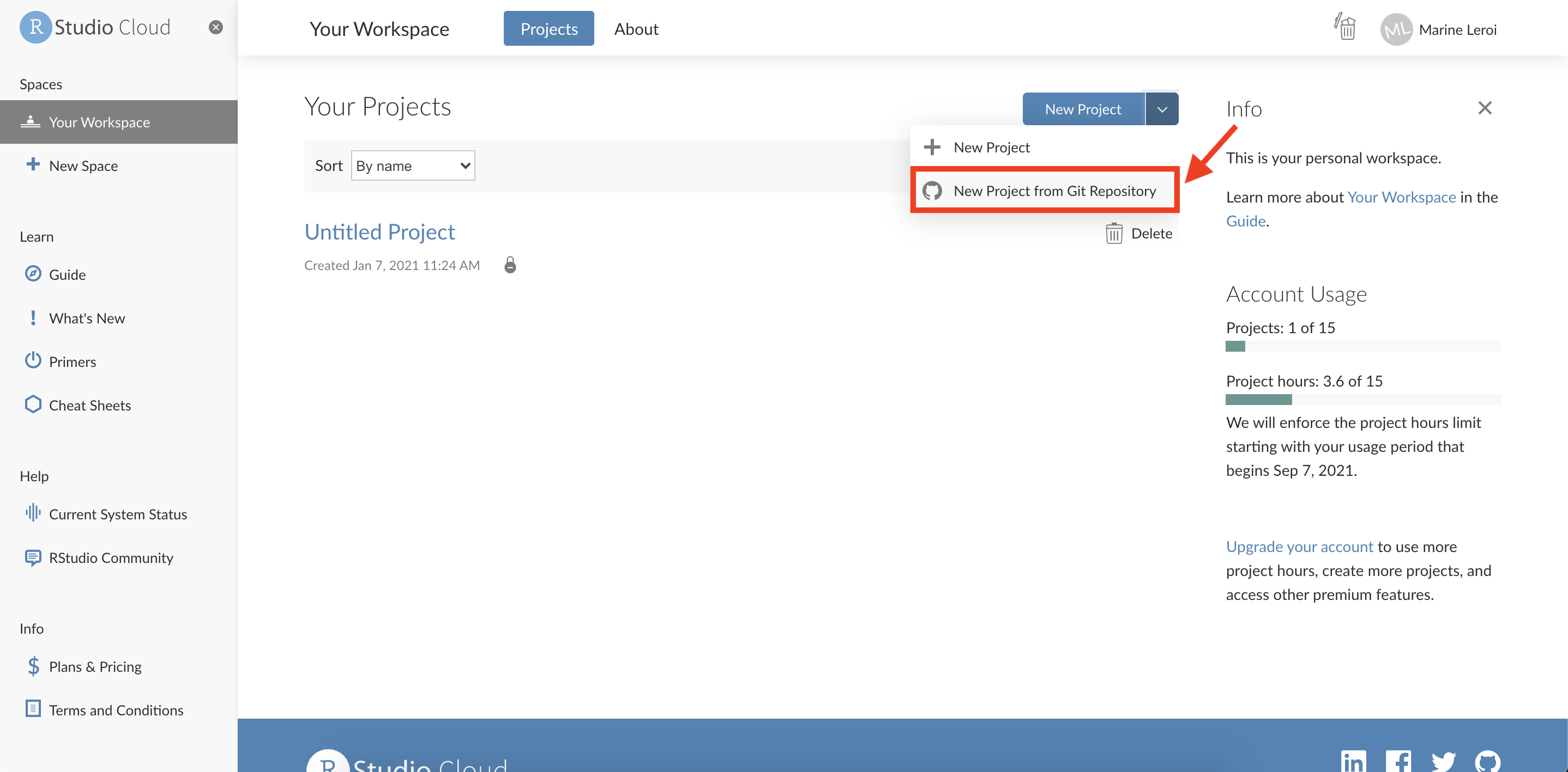{width=600}After creation, in the top-right of RStudio, you should see that Git tab we mentioned becomes active (because this project is now a Git repository). The README.md file should be listed in the Files pane.Now your RStudio project is linked with GitHub. The next steps are to bring your existing work into this repo, and then learn the Pull/Commit/Push cycle.**(If you started from scratch by cloning, you may not have your R Markdown file here yet. You can upload it or create a new one in this project and copy over content. Alternatively, you could have initiated Git in an existing project and connected to GitHub – but that’s a slightly more advanced workflow. For now, it’s fine to bring your work into this new Git project manually.)**### Using a Consistent Naming Convention for FilesBefore we commit files to Git, one best practice: adopt a consistent naming scheme for your files. The book (and many developers) recommend **lower camel case** (also known as **lowerCamelCase**) for file names. This means:* Use all lowercase for the beginning of the filename.* If the name has multiple words, do not use spaces. Instead, concatenate the words and capitalize each subsequent word.* For example, instead of naming a file *“Reproducible Document 1.Rmd”* (which has spaces and capital letters scattered), name it `reproducibleDocument1.Rmd`. Another example: `dataCleanup.R` or `salesAnalysis.Rmd`.Why? Spaces in filenames can cause issues in URLs or require quoting in code. Using a consistent style like lowerCamelCase or snake_case (words_separated_by_underscores) avoids these problems. The key is no spaces, no special characters (stick to letters, numbers, underscores, hyphens, or camelCase caps), and make it readable. LowerCamelCase has the advantage that each word boundary is still clear (because of the capital), without needing an underscore.So as you create files (scripts, data files, images, etc.), name them clearly and consistently. This will pay off when referring to them in code and when collaborating, because there’s no ambiguity or need for awkward quotes around file paths.### The Git Workflow: Pull, Commit, PushWith your project now under Git version control and linked to GitHub, let’s outline the basic workflow. The three main operations you will use constantly are:* **Pull**: Get the latest changes from the remote GitHub repository down to your local project.* **Commit**: Save (record) a snapshot of your changes in the local repository.* **Push**: Send your committed changes up to the remote GitHub repository.Think of it this way: Git is like a journal of changes. You write in the journal locally (commit) and later publish those changes to the world (push). Conversely, if others have written new entries (commits) to the shared journal on GitHub, you pull them to get up-to-date.The mantra to remember, especially when collaborating or even if you work on multiple computers, is: **Pull first, then commit and push.** Always pull at the start of your session to make sure you have the latest version, then do your work, commit your changes, and push them back.Let’s go step by step, using RStudio’s Git interface:1. When you open your RStudio project (e.g., at the start of the day or when you know someone else may have pushed changes), click the **Pull** button. This fetches any changes from GitHub and merges them into your local files. If no one else changed anything, this might not bring any new changes, but it never hurts to pull. If there were changes (for example, maybe the instructor pushed a correction to an exercise or your teammate added data), those files will be updated in your project. In RStudio’s Git tab, the Pull button usually looks like a downward blue arrow.{width=600}2. After pulling (or if no changes needed pulling), you work on your files as usual: edit the R Markdown, maybe add some data or images to your project folder, etc.3. Once you have made some progress and want to save a version, you will **commit** your changes. In the Git tab, you should see a list of files that have been modified, added, or deleted. New files will be marked with `?` (untracked), modified ones with `M`, etc. * Click the checkboxes next to the files you want to include in this commit (or click the **Stage** button to stage selected files). Staging just means “prepare these files to be committed”. Typically, you stage all the files relevant to the change you are committing. * Once staged, those files will move into the "Staged" section in RStudio’s Git interface. * Now click **Commit**. A new window will pop up showing the changes (it may show a diff – lines added/removed in each file). * Enter a **commit message** in the box. This is a short description of what you did, like “Drafted introduction and added images” or “Fixed typo in Markdown section” or “Added ggplot2 visualization of sales data”. A good commit message is clear and specific to the changes made. * Then confirm the commit. The changes are now recorded in your local repository’s history. (At this point, it’s not yet on GitHub – that requires a push.)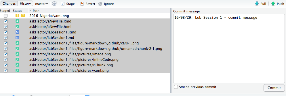{width=600} After committing, the files will no longer show as modified in the Git tab (until you edit them again).4. Finally, **Push** your commit(s) to GitHub. Click the **Push** button (it’s usually an upward arrow). If this is the first time pushing to this repository from your machine, you might be prompted for your GitHub credentials or a PAT (Personal Access Token) since GitHub requires authentication. Follow the prompts (you might need to use a token instead of your password if asked – GitHub has guidance on that, but RStudio might handle it via a one-time setup). On RStudio Cloud, the authentication might be managed automatically via your linked account. When you push, your commits are sent to the GitHub server and incorporated into the remote repository. If someone looks at the GitHub repo page now, they will see your new commits and updated files.If at any point someone else pushed changes while you were working, your push might be rejected because your local is behind. In that case, you should Pull again (to merge their changes) and then push. Usually if you commit first and then try to push and it fails, doing a Pull will bring the other changes and often merge automatically (unless you both edited the same lines, causing a conflict). Git will notify you of conflicts if any, which you’d have to resolve manually (outside the scope of this intro, but basically you’d open the conflicted file, decide which version of lines to keep, then commit the resolved file).For our use (student syncing with instructor’s repository, for example), the typical pattern is:* Always **Pull** when you start working or before you make big changes, to get any updates (e.g., maybe we provided a new dataset or corrected a typo in the starter code).* Work on your tasks.* **Commit** your changes locally with a message about what you did.* **Push** to upload your work to GitHub (so the instructor can see it, or just to back it up for yourself).If you remember "**Pull > Commit > Push**" as a habit, you’ll avoid many common pitfalls like merge conflicts or accidentally diverging from the main repository.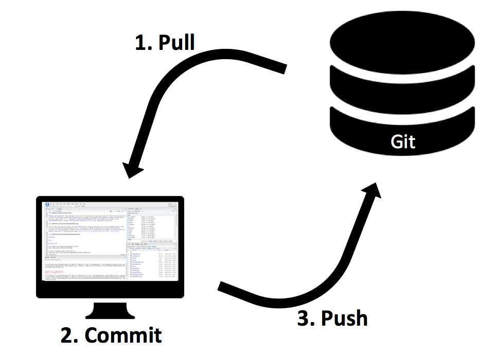{width=600}One more thing: The first time you try to commit in a new Git repo on RStudio, you might get a message that your identity is not set. Git needs to know a name and email to associate with your commits (this can be anything, but typically you use the same email as your GitHub account and your actual name or alias). You set this up once:**Git config (only needed once):** In RStudio, you can open the Terminal (there’s a Terminal tab next to Console, or use Tools -> Terminal -> New Terminal). At the `$` prompt, type the following (replace with your details):```markdowngit config --global user.email "your-email@example.com"git config --global user.name "Your Name"```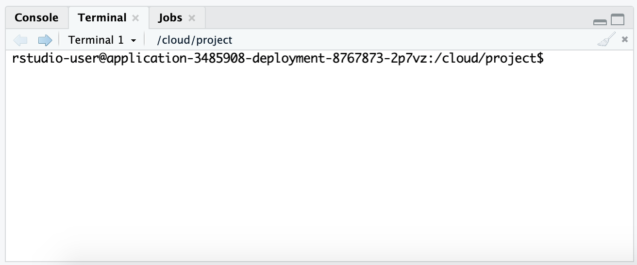{width=600}Hit Enter after each. This stores your name and email in Git’s global config so it will attach them to commits. (The email is what ties commits to your GitHub account if it matches, but even if not, it’s fine.)After configuring, you can proceed to commit and push normally. You shouldn’t have to do this again on the same system.To summarize the **Git workflow**:* **Pull:** Download and integrate changes from GitHub to your local project.* **Stage + Commit:** Select the changes you made and record them as a new version in your local repository with a message.* **Push:** Upload your new commits to the GitHub repository so others (or your other devices) can see them.This will ensure your work is versioned and backed up. No more “final_report_v7_final_FINAL.docx” files – Git will handle versioning seamlessly.**TL;DR** – *Git and GitHub Basics*:* **Git** is a version control system for tracking changes in your files, and **GitHub** is an online hosting service for Git repositories.* Use a consistent naming scheme (like lowerCamelCase) for files to avoid issues and keep things tidy.* The main commands in daily use: * **Pull:** always do this first to get the latest changes from the remote (GitHub). * **Commit:** save your changes locally with a descriptive message. * **Push:** send your committed changes to the remote repository.* Remember the order **Pull → Commit → Push** whenever you start and finish a work session.With your project now under version control, you can collaborate easily and have peace of mind that your work is safe and trackable. Next, we will ensure that even your references and citations in the report are handled in a reproducible way!## Managing References and Citations with ZoteroFinally, we come to a crucial aspect of report writing: citing sources and managing references. In academic or professional reports, you often need to refer to articles, papers, websites, or other sources. Keeping track of these manually can become tedious and error-prone, especially when formatting citations and bibliographies according to specific styles.We will use **Zotero**, a popular free and open-source reference management tool, to handle our references. Zotero allows you to collect references (from academic papers, books, web pages, etc.), organize them, and then easily insert citations into your documents. Combined with an RStudio add-in called **citr** and the **BibTeX/BibLaTeX** system, this becomes a powerful, reproducible way to manage references.Why manage references programmatically? Two big reasons:1. **Efficiency:** Once you have a reference in Zotero, you can cite it in any document with a couple of clicks, and Zotero will handle the heavy lifting of creating and formatting the bibliography. If you need to switch citation styles (say from APA to Chicago), it’s a matter of changing a setting, not retyping everything.2. **Reproducibility:** By keeping a bibliography file (usually `.bib` for BibTeX) under version control with your project, anyone else with your project can compile your document and get the same references and citations. It also means you can regenerate the document at any time and have the citations update or remain consistent.Let’s walk through setting up Zotero and integrating it with R Markdown.### Zotero: Installation and SetupIf you haven’t already, download and install Zotero from the official site: [**Zotero Download**](https://www.zotero.org/download/){target="_blank"}. Zotero is available for Windows, Mac, and Linux. Install the application.Also, install the **Zotero Connector** for your web browser (available on the same download page). This is an extension that allows you to quickly save references to Zotero as you browse (for example, when you’re viewing a journal article, you can click the connector button and it will grab the citation info and even the PDF, if available, into your Zotero library).Open Zotero on your computer. It has a left pane (collections and library organization), a middle pane (list of references), and a right pane (details of the selected reference). You might want to create a new **Collection** for this project or course (think of collections as folders or playlists of references). For example, make a collection called "DPR Project References".You can add references to Zotero manually, or via the connector while browsing. For now, just ensure Zotero is installed and running.### Better BibTeX for ZoteroBetter BibTeX (often abbreviated as **BBT**) is a Zotero plugin that supercharges Zotero’s ability to work with LaTeX/BibTeX and by extension R Markdown. It offers features like stable citation keys (so that the keys used to cite items don’t randomly change), and an auto-export function that keeps a `.bib` file updated with your library or a specific collection.Install Better BibTeX by downloading the latest release (.xpi file) from its GitHub releases page: [**Better BibTeX latest release**](https://github.com/retorquere/zotero-better-bibtex/releases/latest){target="_blank"}. Look for an `.xpi` file (Zotero plugins use this extension).Once downloaded, in Zotero go to **Tools > Add-ons**. In the Add-ons Manager, click the gear icon and choose **"Install Add-on From File..."**, then select the `.xpi` file you downloaded. Confirm to install, and then restart Zotero when prompted.After restarting, Zotero will have Better BibTeX enabled. You can check its presence by going to **Edit > Preferences > Better BibTeX** (or sometimes in a separate tab in the Preferences). There you can configure things like citation key format. The default key format might be something like `[auth][year]` which results in keys like `Wickham2016` for a reference by Wickham in 2016, for example. You can customize it, but default is fine to start.One important thing to do now: set up auto-export of a BibTeX file. This will allow your R Markdown document to always pull citations from your Zotero library without manual exporting each time.* In Zotero, go to **File > Export Library...** (or right-click a specific collection and choose Export).* In the export dialog, choose **Better BibTeX** as the format.* Check the box **“Keep updated”** if available (this is a BBT feature; it will keep the exported file updated as your library changes).* Choose a location and name for the `.bib` file. For example, you might create a file called `references.bib` in your project folder (you can save it directly to your project directory on your computer). If you are on RStudio Cloud, a bit trickier – you might instead periodically export and upload the bib file, or use a synced storage like Dropbox. But let’s assume local for now.* Now, whenever you add or modify references in Zotero, this `references.bib` will be automatically updated by BBT.If “Keep updated” isn’t visible (it might be only when exporting a Collection vs the whole library, can vary by version), alternatively you can periodically re-export. But BBT usually has an option under Preferences -> Automatic Export where you can configure it.Why all this? Because our R Markdown document will use that `.bib` file to retrieve citation info for rendering the bibliography.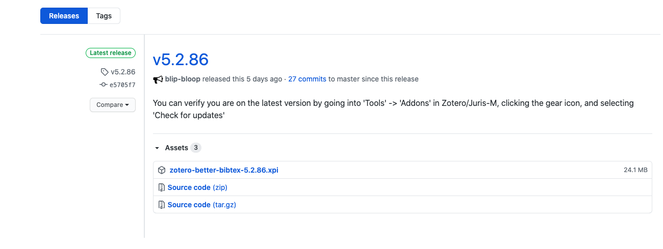{width=500}*(The image above might show the GitHub release page where the .xpi can be downloaded.)*### Configuring the R Markdown YAML for CitationsEarlier we discussed YAML for title, author, etc. To enable citations, we need to add a couple of fields to the YAML:* `bibliography:` – this should point to your `.bib` file (for example, `bibliography: references.bib`).* `csl:` or `biblio-style:` – this is for specifying the citation style. There are two ways to handle style: * If using the default Pandoc citation processor (which is sufficient for most cases), you can specify a CSL (Citation Style Language) file. For example, you might have `csl: apa.csl` for APA style (you’d need to have that csl file downloaded). Alternatively, * If using BibLaTeX via the LaTeX engine (which happens when outputting to PDF with `citation_package: biblatex`), you can use `biblio-style:` to name a BibLaTeX style.* `citation_package: biblatex` – if outputting to PDF, many recommend using the biblatex package for better Unicode support, etc. In our example, we will indeed use PDF as an example and BibLaTeX.Basically, to cover all bases, you can include:```yamlbibliography: references.bibbiblio-style: apaoutput:pdf_document:citation_package: biblatex```This YAML snippet says:* Use `references.bib` for citation data.* When using biblatex (which we will for PDF), use the “apa” style (APA style citations). We could put another style name if desired (like `chicago-authordate` etc., if the LaTeX package is available).* Use biblatex for handling citations in the PDF output.For HTML output, the `biblio-style` might not do anything; instead, Pandoc will look for a CSL file if provided, or default to something like Chicago author-date. If you want a specific style in HTML, you would use a CSL. You could add `csl: apa.csl` (after obtaining the appropriate CSL file from somewhere like Zotero’s style repository).For simplicity, let’s assume APA style for now. If you don’t have the CSL, the above might still produce a default author-year style.So your YAML might now look like:```yaml---title:"My Analysis Report"author:"Jane Doe"date:"2025-06-26"output:pdf_document:citation_package: biblatexbibliography: references.bibbiblio-style: apa---```*(If you’re knitting to HTML, you could instead do `output: html_document` and maybe include a `csl` line. But to keep things consistent, we can keep the YAML as above; it won’t break HTML output, it just might not use the `biblio-style` in that case.)*This YAML setup ensures that when you knit your document:* It knows to look into `references.bib` for any citation keys you use.* It will format the bibliography at the end according to APA style (for PDF via biblatex).* It will include in-text citations in APA format (e.g., parenthetical author-year).### Inserting Citations in R Markdown (with the citr Add-in)Now comes the fun part: actually citing something in your text. You could do this manually by knowing the citation key for an item and typing it, but there’s a handy tool to avoid leaving the RStudio environment: the **citr** add-in.**Installing citr:** citr is an R package that provides an RStudio Add-in. To install it, we actually need the development version from GitHub (though CRAN might have a version; the instructions given in our material use GitHub). Let’s follow those:Open the RStudio Console (or a chunk) and run:```{r}install.packages("devtools")```(This installs the devtools package if you don’t have it, which lets you install packages from GitHub.)Then run:```{r}devtools::install_github("crsh/citr")```This will download and install the citr package from GitHub. It might ask you to update some packages; if you see a prompt like "These packages need updating, enter 1 for All, etc.", you can enter `1` to accept updating all needed packages.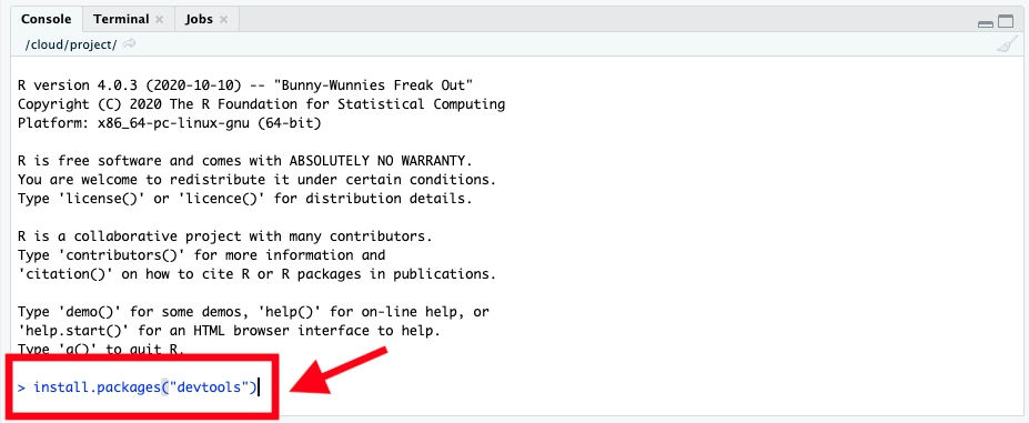{width=700}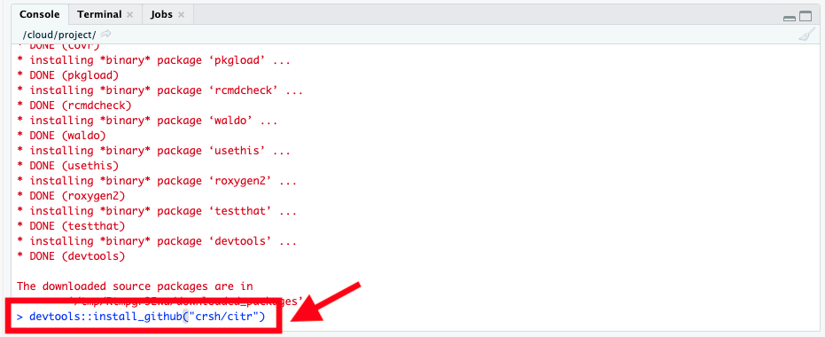{width=700}If during installation you get a prompt in the console (often something about building vignettes or updating packages) like this:```1: All2: CRAN packages only3: None```Just type `1` and press enter to select All, as instructed: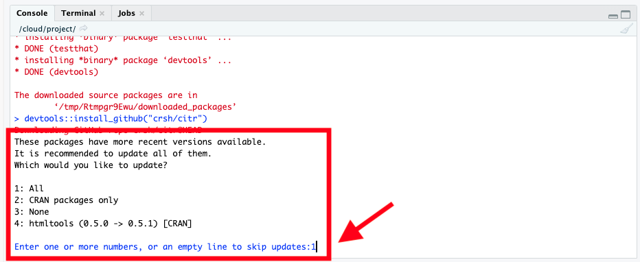{width=700}After installation, it’s a good idea to restart your R session (because you installed new packages). In RStudio, go to **Session > Restart R** (or use the keyboard shortcut: Ctrl+Shift+F10). This ensures the new add-in is registered.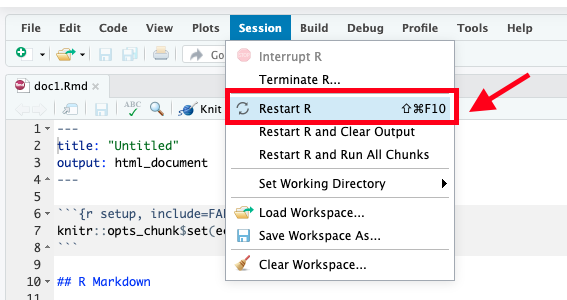{width=550}Now, in RStudio, check the **Addins** menu (it’s typically at the top toolbar, to the left of Help, appearing when you have an R Markdown open or just in general). Click **Addins**, and find **Insert Citations** (you can use the search bar in the addins list to type “citation” and it should filter). This “Insert Citations” add-in is provided by citr.{width=550}When you click **Insert Citations**, a window should pop up. (Note: Zotero must be running, because citr will try to communicate with Zotero to get the references.) In this window, you should see the list of references from your Zotero library or at least those in the exported Bib file. There will be a search bar where you can type an author name, year, title, etc., to filter your references.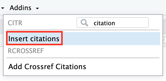{width=300}Select the reference(s) you want to cite (you can usually select multiple by holding Ctrl or Shift, or add them one by one). Once selected, you can press Enter or click "Insert". The add-in will then insert citation keys into your R Markdown document at the cursor position.The syntax that appears will be like `[@citationKey]` for a parenthetical citation or `@citationKey` for an in-text citation, depending on what you chose. By default, citr likely inserts `[@key]` (parenthetical). You can always edit for narrative citations.For example, if you selected an item by James (1890) with citation key `james_1890`, the add-in might insert `[@james_1890]`. In your text, this will render as (James, 1890) in APA style. If you wanted "James (1890)" as part of the sentence, you would remove the brackets: just `@james_1890` in the Rmd will produce James (1890).The add-in is nice because you don’t have to remember or look up the keys; you just search your library.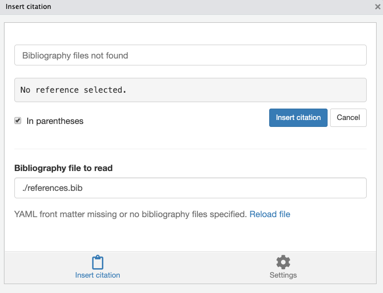{width=550}The pop-up window (image above) shows the references; you can likely double-click or use buttons to insert.After inserting the citation in your R Markdown text, you’ll see the placeholder like \[@james_1890]. If you now knit your document, it will replace that with a formatted citation and add the full reference in a “References” or “Bibliography” section at the end of the document (usually automatically, unless you specify otherwise).By default, the bibliography will appear under a heading like “References” at the end of the document.If for some reason you are not using citr or can’t (maybe working on a machine where you can’t install it), you can still cite by typing the keys manually. The syntax to remember:* `[@key]` for parenthetical (author, year).* `@key` for in-text (Author (Year)).* You can add page numbers or prefixes/suffixes, for example: `[@key, p. 123]` or `[@key, see Chapter 1]`. Also, if you want to suppress the author in parenthetical (say you already mentioned the author’s name in text and just want the year in parentheses), you prefix the key with a minus: `[-@key]` will give just (Year).Here’s a quick reference of citation syntax (assuming your Bib has entries for James 1890 and Bem 2011 with keys as shown):| Citation type | Syntax | Rendered citation || ---------------------------------------------------------- | -------------------------- | ------------------------------------------------------------------------------------------------------------------------ || Citation within parentheses | `[@james_1890]` | (James, 1890) || Multiple citations | `[@james_1890; @bem_2011]` | (Bem, 2011; James, 1890) *(order will be automatically sorted by citation style rules, often alphabetically by author)* || In-text citation (no parentheses around author name) | `@james_1890` | James (1890) || Year-only, for narrative citations where author is in text | `[-@bem_2011]` | (2011) *i.e., just the year in parentheses, assuming you wrote “Bem” in text already* |As mentioned, you can add a prefix or suffix within the square brackets:For example, `[@bem_2011, p. 5]` would yield (Bem, 2011, p. 5).Or, `[@bem_2011; @james_1890, Chapter 2]` yields (Bem, 2011; James, 1890, Chapter 2).Each `;` separates citations, and a comma after a key separates the citation from its suffix.One thing to be cautious about: When multiple citations are inside one set of brackets, they will be sorted by the processor. So if you write `[e.g., @james_1890; @bem_2011]`, it may output as (e.g., James, 1890; Bem, 2011) or with authors sorted alphabetically after the text “e.g.,” stays tied to James (maybe not what you intended because you wanted e.g. to apply to both). There’s no easy fix to that except to word your sentences carefully or cite separately. Just a nuance to keep in mind: prefixes belong to the specific citation immediately following them within the brackets.Now, after adding a few citations in your text, try knitting your document. If everything is set up correctly, you should see in-text citations and a reference list at the bottom. If you encounter any errors:* Make sure the YAML is correct (especially indentation – YAML is picky about indentation).* Make sure the .bib file path is correct. If the .bib file is not in the same directory as the .Rmd, adjust the path accordingly, e.g., `bibliography: refs/references.bib` if it’s in a subfolder.* Ensure Zotero is running and BBT is keeping the bib updated (or that you exported the bib after adding references).* If using PDF output and you get an error about biber or something, ensure you have a TeX distribution installed with biber (TinyTeX for example if not already).Once it works, you’ll have fully automated citations in your report!**TL;DR** – *Reference Management Recap*:* Use **Zotero** to collect and manage references for your project. It's free and helps keep all citation info handy.* Install the **Better BibTeX** plugin for Zotero to streamline integration with R Markdown (ensures stable citation keys and easy export).* Configure your R Markdown document’s YAML to point to a `.bib` file (`bibliography:`) and use a citation style (`biblio-style:` or `csl:` and possibly `citation_package: biblatex` for PDF).* Install and use the **citr** add-in in RStudio to search and insert citations without leaving the editor.* In citations: use `@citekey` for in-text and `[@citekey]` for parenthetical. Add multiple inside one set of brackets separated by semicolons for combined parentheses.* The reference list will be generated automatically upon knitting, listing all sources you cited.### Getting Your Hands Dirty: Citing Sources in Your ReportLet’s extend the earlier exercise. You had reproduced a sample report in Markdown. Now, suppose we provide you with a BibTeX file of references (say `sample_refs.bib`) and an updated version of the report that includes citations. Your task:1. Add the necessary YAML fields to your document to enable citations (point to the provided `.bib` file, specify the style).2. Insert the citations in the text at the appropriate places exactly as in the target report (you can use citr with the provided bib, or if you know the keys, type them).3. Include the bibliography in the output (it will happen automatically when you knit if YAML is correct).The folder named *chapter4* on the [GitHub repository](https://github.com/warint/DPR/tree/main/chapter4){target="_blank"} contains the `.bib` file and an example of the report with references. Use those to guide you.After knitting, your output should match the [**report with references**](https://warin.ca/sessions/exercises/dpr/chap4/chap4-managing-references.html){target="_blank"} (which presumably shows the citations and reference list).By completing this, you will have experienced the full workflow: writing in R Markdown, using Git for version control, and adding citations for a polished, professional document. You are now well-equipped to produce a reproducible research report from start to finish!


