knitr::opts_chunk$set(
echo = FALSE,
message = FALSE,
warning = FALSE,
fig.width = 7,
fig.height = 5
)14 Resilience of Global Supply Chains in a Geopolitical Age
The contemporary global economy is organized through dense, multi-tier supply networks that connect firms, logistics systems, standards regimes, and jurisdictions. For three decades, the dominant organizing logic favored lean, globally dispersed architectures that minimized buffers in order to exploit specialization, scale, and cost arbitrage. The succession of disruptions associated with the COVID-19 pandemic, the escalation of U.S.–China trade and technology frictions, and the Russia–Ukraine war has clarified that these architectures embed non-trivial tail risks whose consequences are magnified by concentration, limited substitutability, and information frictions across tiers. A fundamental lesson follows: resilience is not a property of a single firm or site, but an emergent property of a network embedded in legal and geopolitical regimes, where interdependencies, chokepoints, and coordination constraints shape both shock transmission and recovery trajectories (Acemoglu et al. (2012); Carvalho et al. (2021)).
This chapter develops a geoeconomic account of supply chain resilience under geopolitical risk. The argument integrates three complementary lenses. The first is the macroeconomics of production networks, which clarifies why idiosyncratic supplier shocks can generate aggregate outcomes and why the distribution of dependencies matters at least as much as their average level (Acemoglu et al. (2012); Carvalho et al. (2021)). The second is institutional political economy, which specifies how sanctions, export controls, and standards conflict operate as state-contingent constraints that can convert network centrality into leverage, thereby embedding geopolitical rivalry within the microstructure of global commerce (Farrell and Newman (2019)). The third is operations and strategy, which formalizes the efficiency–resilience trade-off and emphasizes that robust designs are typically portfolios combining redundancy, buffers, flexibility, and visibility rather than single levers (Tang (2006); Pettit, Fiksel, and Croxton (2010); Sheffi (2005); Chopra and Sodhi (2014)).
14.1 Conceptual foundations: networks, governance, and resilience metrics
In global supply chains, incomplete contracts and relationship-specific investments generate dependence on a limited number of suppliers, lanes, and certifying authorities. Such dependence is often invisible in normal times because it is masked by stable lead times and routinized compliance. Network theory makes dependence legible by representing supply chains as graphs with nodes (firms, facilities, ports, standards bodies) and edges (supplier relations, transport lanes, contractual interfaces). Two properties are central. Centrality identifies nodes whose failure disproportionately disrupts connectivity; modularity and redundancy determine whether disruptions remain local or cascade through the system. In production networks with skewed input shares and limited substitution, micro shocks can become macro shocks, particularly when they hit “granular” suppliers whose outputs are widely used (Acemoglu et al. (2012)).
Institutional context determines whether alternative paths are feasible. Trade rules, technical standards, licensing regimes, and sanctions compliance are not external parameters; they constitute the feasible set. In a world of geopolitical rivalry, the feasible set can change discontinuously. Export controls on advanced semiconductors, restrictions on dual-use items, and sanctions on shipping, insurance, and payments can make a technically possible reallocation legally infeasible. The framework of weaponized interdependence clarifies why such constraints are strategically potent: states positioned at nodal infrastructures can use jurisdiction and standard-setting capacity to influence flows across the network (Farrell and Newman (2019)).
Operationalizing resilience requires metrics that capture both resistance and recovery. Let (Q(t)) be a normalized performance index for a focal supply chain. A common area-based metric defines resilience over \([t_0,t_1]\) as \(R = 1 - \frac{1}{t_1-t_0}\int_{t_0}^{t_1}[1-Q(t)],dt\). This measure rewards shallower performance drops and faster recovery, and it can be complemented by time-to-survive and time-to-recovery concepts widely used in practice. The following code computes a discrete approximation to the area-based index under simulated recovery paths.
# $resilience_index
# [1] 0.832
The conceptual point is not the specific functional form, but the mapping from network structure and governance constraints to (Q(t)). Identical shocks can yield different (Q(t)) trajectories across firms and sectors because substitutability, compliance constraints, and reconfiguration capacity differ.
14.2 Geopolitical risk as a structured shock process
Geopolitical risk differs from ordinary operational risk in three respects. First, it is often discontinuous, changing the feasible set rather than incrementally changing costs. Second, it is frequently targeted, exploiting chokepoints and jurisdictional reach rather than arising randomly. Third, it is strategic, meaning that actors anticipate and respond to each other, so the environment is endogenously shaped by adaptation.
This motivates a shift from treating disruptions as independent failures toward treating them as scenario families. A useful empirical complement is the Geopolitical Risk (GPR) index, which measures time variation in geopolitical tensions using newspaper text and has been used to study macroeconomic effects of geopolitical events (Caldara and Iacoviello (2022)). In a supply chain context, such indices can be integrated as regime indicators: when geopolitical risk rises, correlations between supplier failures rise, and the value of redundant jurisdictions increases.
14.3 Targeted fragility and the logic of chokepoints
Recent disruptions highlight the difference between random fragility and targeted fragility. Random failures degrade performance through dispersed disruptions; targeted disruptions exploit centrality. Export controls, sanctions on dominant suppliers, closure of key ports, restrictions on payment infrastructures, and denial of insurance services are all targeted mechanisms that can induce discrete fragmentation rather than gradual degradation.
The following code constructs a stylized network and highlights potentially critical nodes by centrality. The network is synthetic, but the diagnostics mirror real supply mapping exercises.
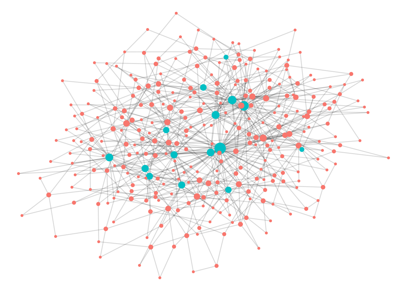
A canonical experiment compares random removals with targeted removals of high-centrality nodes. In real-world terms, random removals approximate dispersed disruptions; targeted removals approximate the loss of a dominant supplier, a sanctioned intermediary, or a closed corridor. The following is kept as a dormant template to preserve readability.
# [1] 300
#  [1]  0  5 10 15 20 25 30 35 40 45 50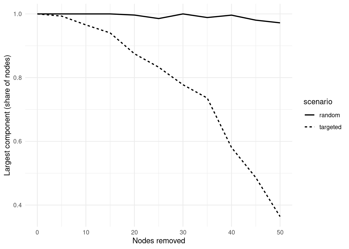
The geoeconomic implication is that resilience investments must be structured around specific chokepoints and jurisdictions. A firm can diversify suppliers but remain fragile if all suppliers depend on the same transit corridor, certification regime, or sanctions-exposed intermediary.
14.4 Measuring dependence: concentration, substitutability, and jurisdictional exposure
Concentration on a single supplier, partner, or corridor increases expected disruption loss. A parsimonious descriptive metric is the Herfindahl–Hirschman Index (HHI) computed over partner shares. The example below contrasts a baseline configuration with a simple reallocation that reduces dependence on a dominant partner.
# # A tibble: 2 × 2
#   configuration   HHI
#   <chr>         <dbl>
# 1 Baseline      0.375
# 2 Rebalanced    0.272
The HHI becomes strategically meaningful when linked to substitution. Substitution is not only technological; it is also legal and organizational. A supplier is not substitutable if switching requires recertification, redesign, or is blocked by export controls. In this sense, “jurisdictional exposure” is an additional dimension of dependence: suppliers embedded in the same compliance perimeter may fail jointly even if operationally independent.
The Monte Carlo illustration below clarifies why, absent perfect correlation, multi-sourcing reduces severe shortfall risk, even if the marginal supplier is not uniformly less risky.
# # A tibble: 2 × 2
#   configuration prob_shortfall_below_50pct
#   <chr>                              <dbl>
# 1 Concentrated                       0.121
# 2 Diversified                        0.119
In geopolitical shocks, correlations typically rise because multiple suppliers can be affected simultaneously by the same policy perimeter, by the same corridor disruption, or by the same financial restriction. This shifts the resilience problem away from simple supplier counts toward diversity of jurisdictions, lanes, and compliance regimes.
14.5 Sectoral archetypes: why semiconductors, pharmaceuticals, food, and energy behave differently
The mechanisms described above are cross-sectoral, but the resilience problem differs systematically by sector. Semiconductors illustrate extreme capital intensity, long lead times, and high concentration at specific stages of fabrication and equipment supply. Substitution is limited by design specificity and by the need for qualification and yield stabilization. Pharmaceuticals illustrate regulatory and quality constraints that can make “physical” substitution infeasible without time-consuming approval and validation, even when alternative capacity exists. Food systems illustrate a different structure in which logistics, storage, and seasonal constraints interact with climate shocks and export restrictions, often producing price spikes and political instability through distributional effects. Energy systems combine physical infrastructure lock-in with geopolitical constraints, where route dependence and long-lived assets produce persistent vulnerability, and where reconfiguration requires large-scale investment rather than short-run switching.
A geoeconomic reading treats these sectors as distinct regimes of substitutability and governance. The same policy instrument, such as export controls, will have different effects depending on how modular the production process is and how quickly certification and redesign can occur. This is why resilience policy is rarely “one size fits all” and why governments have increasingly treated certain sectors as strategic, engaging in industrial policy and stockpiling, even when such interventions reduce static efficiency.
14.6 The efficiency–resilience frontier and the logic of robust portfolios
Resilience investments impose costs in normal states and deliver benefits in rare states. This creates a classic problem of underinvestment when tail risks generate spillovers that private actors do not internalize. In practice, robust strategies tend to be portfolios rather than single instruments: limited redundancy for critical inputs, buffers calibrated to time-to-survive, flexible capacity, and contract structures that enable priority access under disruption (Tang (2006); Chopra and Sodhi (2014)). A complementary conceptualization frames resilience as the balance of vulnerabilities and capabilities, emphasizing that resilience is jointly determined by exposure and the capacity to respond (Pettit, Fiksel, and Croxton (2010)). The broader managerial literature underscores the importance of preparing for disruptions through flexible logistics and contingency planning, rather than attempting to forecast specific shocks precisely (Sheffi (2005)).
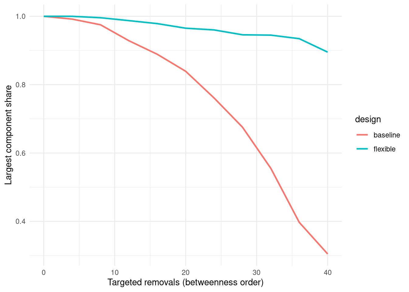
The following stylized simulation shows how modest structural flexibility, represented by a small number of latent backup links, can reduce fragmentation under targeted disruptions. The point is not realism of the network generation, but interpretability of the mechanism.
14.7 Regionalization, friend-shoring, and the governance of modularity
A salient organizational response to geopolitical risk is partial regionalization into semi-autonomous poles, characterized by tighter intra-regional coupling and looser inter-regional bridges. The underlying logic is modularity: if networks are structured into modules linked by limited bridges, disruptions can be contained, and governance can be stabilized within institutional zones. Friend-shoring is a related concept that emphasizes reducing exposure to adversarial policy shocks by concentrating reliance on lower-tension jurisdictions. These strategies are not equivalent to deglobalization. They represent a re-optimization of interdependence under higher variance and higher policy risk.
Institutional arrangements condition the feasibility and cost of modularity. Trade agreements, mutual recognition, customs facilitation, and credible dispute settlement expand the feasible set for diversification and rerouting; sanctions regimes and standards conflict shrink it. In this sense, resilience is jointly produced by firms and institutions. Where institutional capacity is high and rules are credible, the cost of reconfiguration falls; where governance is uncertain, private actors face higher option costs and a narrower set of feasible contingencies.
14.8 Visibility, coordination, and the political economy of information
Supply chain disruptions are frequently amplified by information frictions. Firms commonly lack visibility beyond first-tier suppliers; governments may lack timely information about inventories and bottlenecks; logistics systems may have delayed and noisy signals about congestion. Improving visibility changes the dynamics of recovery by enabling prioritization and coordinated rerouting. However, visibility is also political economy: information is a strategic asset, and incentives to share it are limited when it reveals bargaining positions or compliance vulnerabilities. As a result, public–private coordination becomes a governance problem. The state’s role is not only to impose buffers but to create credible frameworks for information sharing, crisis coordination, and targeted support that reduce collective-action failures.
14.9 Conclusion
In a geopolitical age, supply chain design must internalize the possibility of targeted, policy-induced disruptions that exploit network structure. The production-network literature clarifies why localized shocks can produce aggregate outcomes through propagation and amplification mechanisms that depend on topology and substitutability (Acemoglu et al. (2012); Carvalho et al. (2021)). The institutional literature clarifies why geopolitical rivalry converts network position into leverage and why legal-jurisdictional dependence is itself a resilience variable (Farrell and Newman (2019)). The operations literature clarifies why mitigation is best treated as a portfolio problem: calibrated redundancy, buffers, contingent capacity, and coordination capabilities shift the efficiency–resilience frontier in a cost-disciplined manner (Tang (2006); Pettit, Fiksel, and Croxton (2010); Chopra and Sodhi (2014); Sheffi (2005)).
Resilience, in this framework, is engineered substitutability under strategic rivalry. The objective is not autarky, but architectures and governance arrangements that reduce the probability that a small number of chokepoints—physical, organizational, or jurisdictional—can generate systemic disruption and that enable faster recovery when disruptions occur.
Appendix: minimal helper for an area-based resilience index
# [1] 0.75