Table of Contents
Pedagogical Material
As part of the Hacking Health Covid-19, the SKEMA Global Lab in AI provided to SKEMA’ students a fully developped data science environment to realize their project. See [here].
For this specific module, this team used these following courses:
- Module 1: Data Visualizations
- Module 4: Predictive Modelling
- Module 6: Mapping
Project Presentation
When an epidemic occurs, timely information on the extent of the spread and the number of people infected is an important prerequisite for the development of prevention programmes. If the number and extent of cases are not known in time, the immediate consequence is the spread and re-proliferation of the virus. I think one of the main reasons for today’s situation is the lack of realistic and intuitive understanding of the situation at the beginning of the year, which has led to some disregard for the development of the epidemic.
Therefore, in the scenario of real-time surveillance of the epidemic, visualization is a very important element in addition to the realism and real-time nature of the data. We see today that in some countries where data science is not well developed, the daily epidemic releases of the National Health Construction Commissions are still in the form of textual descriptions, which can result in untimely and incomprehensible information delivery. We also use data visualization as a weapon to predict inflection points and make predictions about the economies of countries affected by the epidemic, and humanity can finally overcome this disaster
Our goal is to create a heatmap to demonstrate the impact of Covid-19 on national economies and we also want to predict the inflection point of the epidemic.
The design of the Workflow is as follow:
Technical Process
First, we need to download libraries, below are the libraries that we need to use inthe process.
library(readxl)
library(ggplot2)
library(sf)
library(rnaturalearth)
library(ggmap)
library(flexdashboard)
library(kableExtra)
library(dplyr)
After downloading the packages, we have a first view of the data. We found that thereare a lot of missing values, so the dataset need to be cleaned.
# To load the data
covid <- read_excel("./data/covid-fci-data.xlsx")
For cleaning the data, we replace all the missing values by NA, and remove all of them.
#finding the missing values
sum(is.na(covid))
[1] 0
covid$LAT[covid$LAT==""] <- NA
mean(covid)
[1] NA
#storing the level 1 policy as policy1 and replacing the missing values with NA
policy1=as.factor(covid$`Level 1 policy measure`)
covid$`Level 1 policy measure`[covid$`Level 1 policy measure`==""] <- NA

income=covid$`Level of income`
date=as.factor(covid$`Entry date`)

#storing the level 1 policy as policy1 and replacing the missing values with NA
policy2=as.factor(covid$`Level 2 policy measure`)
covid$`Level 2 policy measure`[covid$`Level 2 policy measure`==""] <- NA

#remove the missing values
covid <- na.omit(covid)
After removing all the missing data, we got the clean data that we can use forvisualization. Below is the result after cleaning.
kable(head(covid))| Iso 3 Code | Level of income | Region | Country | Date (at or prior to) | Entry date | Level 1 policy measure | Level 2 policy measure | LAT | LONG |
|---|---|---|---|---|---|---|---|---|---|
| CHN | Upper middle income | EAP | China | 2020-02-01 | 2020-03-21 | Financial Institutions | Operational continuity | 31.8257 | 117.2264 |
| CAN | High income | Other G20 | Canada | 2020-02-03 | 2020-03-21 | Financial Markets | Market functioning | 53.9333 | -116.5765 |
| THA | Upper middle income | EAP | Thailand | 2020-02-05 | 2020-03-21 | Liquidity/funding | Policy rate | 15.0000 | 101.0000 |
| BLR | Upper middle income | ECA | Belarus | 2020-02-19 | 2020-03-31 | Liquidity/funding | Liquidity (incl FX)/ELA | 53.7098 | 27.9534 |
| BLR | Upper middle income | ECA | Belarus | 2020-02-19 | 2020-03-31 | Financial Markets | Market functioning | 53.7098 | 27.9534 |
| BLR | Upper middle income | ECA | Belarus | 2020-02-19 | 2020-03-31 | Liquidity/funding | Policy rate | 53.7098 | 27.9534 |
Plotting the data, by using ggplot, we can have a view of every country. The below dot plots show the level of income of various countries with respect to different policies they implemented in time to fight against COVID-19.
#ploting the cointries with respect to policy1 and income
ggplot(covid, aes(Country,date, color = policy1)) +
  geom_point(aes(shape = income), size = 3) +
  theme(text = element_text(size=6),
        axis.text.x = element_text(angle = 90, hjust = 1))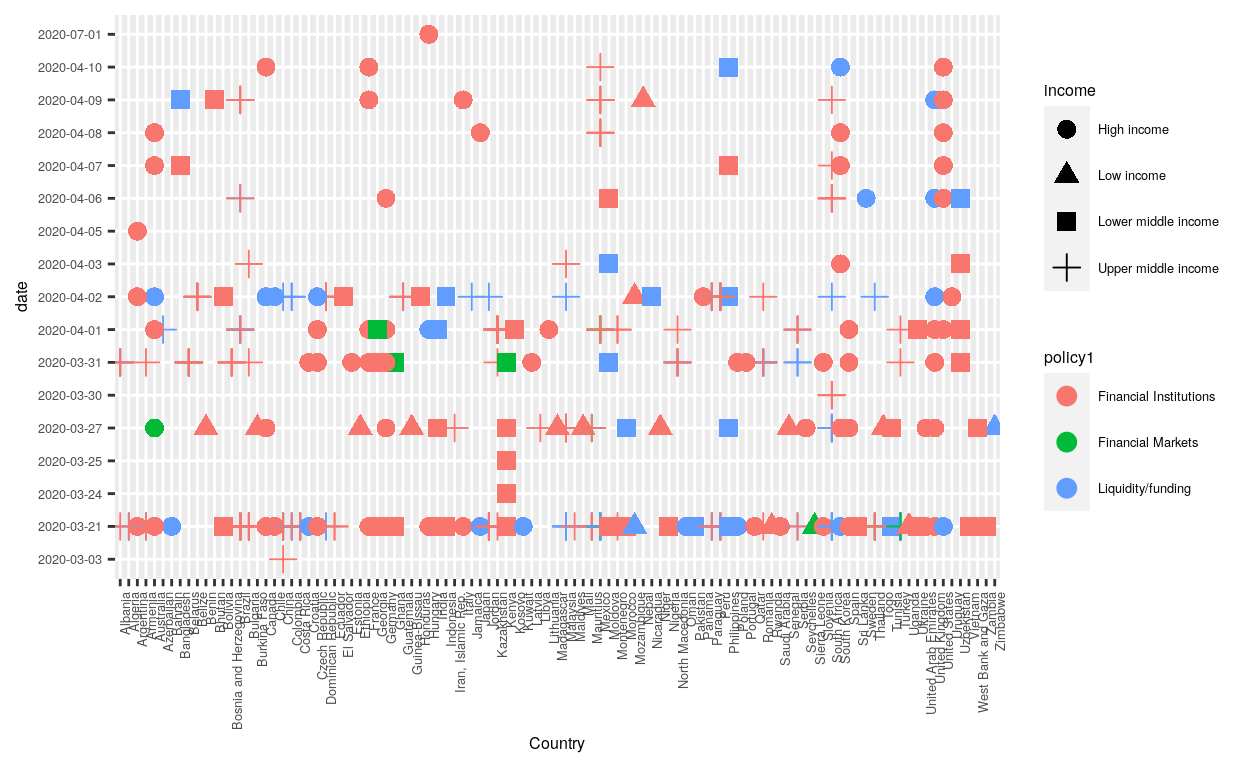
#ploting the cointries with respect to policy1 and income
ggplot(covid, aes(Country,date, color = policy2)) +
  geom_point(aes(shape = income), size = 3) +
  theme(text = element_text(size=6),
        axis.text.x = element_text(angle = 90, hjust = 1))
By using the packahes rnaturalearth and rnaturalearthdata we can have a global viewof the data.
world <- map_data("world")
world <- filter(world, region != "Antarctica")

#mapping policy1
ggplot() +
  geom_polygon(data = world, aes(x = long, y = lat, group = group), fill = "gray", color = "black", size = .3) +
  geom_point(data = covid, aes(x = LONG, y = LAT, fill = policy1), size = 2, shape = 23)
#mapping policy2
ggplot() +
  geom_polygon(data = world, aes(x = long, y = lat, group = group), fill = "gray", color = "black", size = .3) +
  geom_point(data = covid, aes(x = LONG, y = LAT, fill = policy2), size = 2, shape = 23)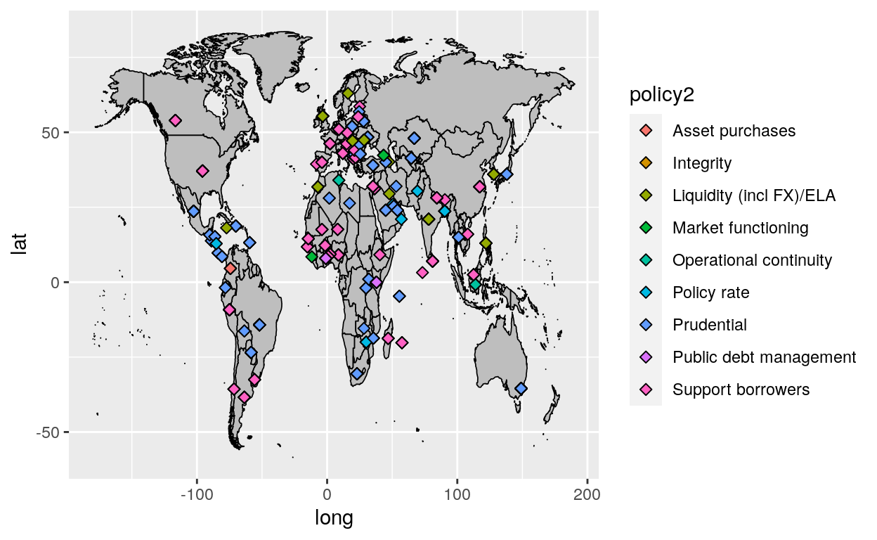
First of all, we would like to thank SKEMA quantum AI Lab for giving us a chance to truly understand covid-19 with the method of data scientific analysis. Through this project, we realize the high efficiency and strong readability of data visualization for solving practical problems, but at the same time, we also recognize that data visualization is not a “Silver Bullet”, Because of the source and authenticity of the data itself, the results of data visualization will be fundamentally different. At the same time, the practical significance behind each number can not be easily displayed by several pictures. As a powerful tool, data visualization can be used to help us understand reality, but it still needs us to be human to make the final decision, in some cases, it is impossible to exclude some countries from making the data “Say what their citizens want to hear” for political reasons.
tl;dr
library(readxl)
library(ggplot2)
library(sf)
library(rnaturalearth)
library(ggmap)
library(flexdashboard)
library(kableExtra)
library(dplyr)

# To load the data
covid <- read_excel("./data/covid-fci-data.xlsx")

#finding the missing values
sum(is.na(covid))
covid$LAT[covid$LAT==""] <- NA
mean(covid)

#storing the level 1 policy as policy1 and replacing the missing values with NA
policy1=as.factor(covid$`Level 1 policy measure`)
covid$`Level 1 policy measure`[covid$`Level 1 policy measure`==""] <- NA

income=covid$`Level of income`
date=as.factor(covid$`Entry date`)

#storing the level 1 policy as policy1 and replacing the missing values with NA
policy2=as.factor(covid$`Level 2 policy measure`)
covid$`Level 2 policy measure`[covid$`Level 2 policy measure`==""] <- NA

#remove the missing values
covid <- na.omit(covid)

kable(head(covid))

#ploting the cointries with respect to policy1 and income
ggplot(covid, aes(Country,date, color = policy1)) +
  geom_point(aes(shape = income), size = 3) +
  theme(text = element_text(size=6),
        axis.text.x = element_text(angle = 90, hjust = 1))

#ploting the cointries with respect to policy1 and income
ggplot(covid, aes(Country,date, color = policy2)) +
  geom_point(aes(shape = income), size = 3) +
  theme(text = element_text(size=6),
        axis.text.x = element_text(angle = 90, hjust = 1))

world <- map_data("world")
world <- filter(world, region != "Antarctica")

#mapping policy1
ggplot() +
  geom_polygon(data = world, aes(x = long, y = lat, group = group), fill = "gray", color = "black", size = .3) +
  geom_point(data = covid, aes(x = LONG, y = LAT, fill = policy1), size = 2, shape = 23)

#mapping policy2
ggplot() +
  geom_polygon(data = world, aes(x = long, y = lat, group = group), fill = "gray", color = "black", size = .3) +
  geom_point(data = covid, aes(x = LONG, y = LAT, fill = policy2), size = 2, shape = 23)
To go further with our pedagogical platform
- Our Coding School
- Our Potential Modules
- Module 1: Data Visualizations
- Module 2: Data Warehouse
- Module 3: News Collection and Analysis
- Module 4: Predictive Modelling
- Module 5: Social Media Collection and Analysis
- Module 6: Mapping
- Module 7: Bibliometrics
- Module 8: Topic Modelling
- Module 9: Covid-19 and International Flows
- Module 10: Covid-19 and Finance
- Module 11: Covid-19 and Public Policies
- Module 12: Covid-19 and Ethics
- Our Databases and APIs