Table of Contents
Pedagogical Material
As part of the Hacking Health Covid-19, the SKEMA Global Lab in AI provided to SKEMA’ students a fully developped data science environment to realize their project. See [here].
For this specific module, this team used these following courses:
- Module 1: Data Visualizations
- Module 4: Predictive Modelling
Project Presentation
In order to realize our project, we used the John Hopkins data to create a predictive model. Based on the ARIMA model, we selected the United States to do a time series analysis on the evolution of Covid-19 cases and deaths.
Technical Process
# Load packages
library(tidyverse)
library(lubridate)
library(rvest)
library(stringdist)
library(forecast)
Step 1: Pulling and tidying the Johns Hopkins Covid-19 data to long format
We need to build a function to read .csv files and convert them to long format. Next, we pull official country level indicators from the UN Statistics Division to get country level identifiers. Merging by country name is messy. I start with a fuzzy matching approach by using the stringdist package.
We took the data cleaning and engneering [here]
# Function to read the raw CSV files
# Files are aggregated to the country level and then converted to long format.
clean_jhd_to_long <- function(df) {
  df_str <- deparse(substitute(df))
  var_str <- substr(df_str, 1, str_length(df_str) - 4)

  df %>% group_by(`Country/Region`) %>%
    filter(`Country/Region` != "Cruise Ship") %>%
    select(-`Province/State`, -Lat, -Long) %>%
    mutate_at(vars(-group_cols()), sum) %>%
    distinct() %>%
    ungroup() %>%
    rename(country = `Country/Region`) %>%
    pivot_longer(
      -country,
      names_to = "date_str",
      values_to = var_str
    ) %>%
    mutate(date = mdy(date_str)) %>%
    select(country, date, !! sym(var_str))
}

confirmed_raw <- read_csv("https://raw.githubusercontent.com/CSSEGISandData/COVID-19/master/csse_covid_19_data/csse_covid_19_time_series/time_series_covid19_confirmed_global.csv")
deaths_raw <- read_csv("https://raw.githubusercontent.com/CSSEGISandData/COVID-19/master/csse_covid_19_data/csse_covid_19_time_series/time_series_covid19_deaths_global.csv")

jh_covid19_data <- clean_jhd_to_long(confirmed_raw) %>%
  full_join(clean_jhd_to_long(deaths_raw))
Step 2: Selecting a country to analyze
In order to take a country’s data from the DF for analysis, we need to first define a country name variable, and then use this variable, called an indicator, to create a subset and “sample” the country.
We selected the US country to do the time series analysis with ARIMA model.
#select a country to do time series analysis with ARIMA model
slctcountry = "US" #This varible defines the county
countrydata <- subset(jh_covid19_data, country == slctcountry)
Step 3: Converting to ts format and using auto.arima function to analyze
We converts(ts founction) the data frame into time series by using frequency 365 (in days), and it will start with 22nd Jan. 2020. Then we plot it:
#time series analysis for confirmed cases
tscfm <- ts(countrydata$confirmed, frequency = 365.25, start=c(2020,1,22))
plot.ts(tscfm)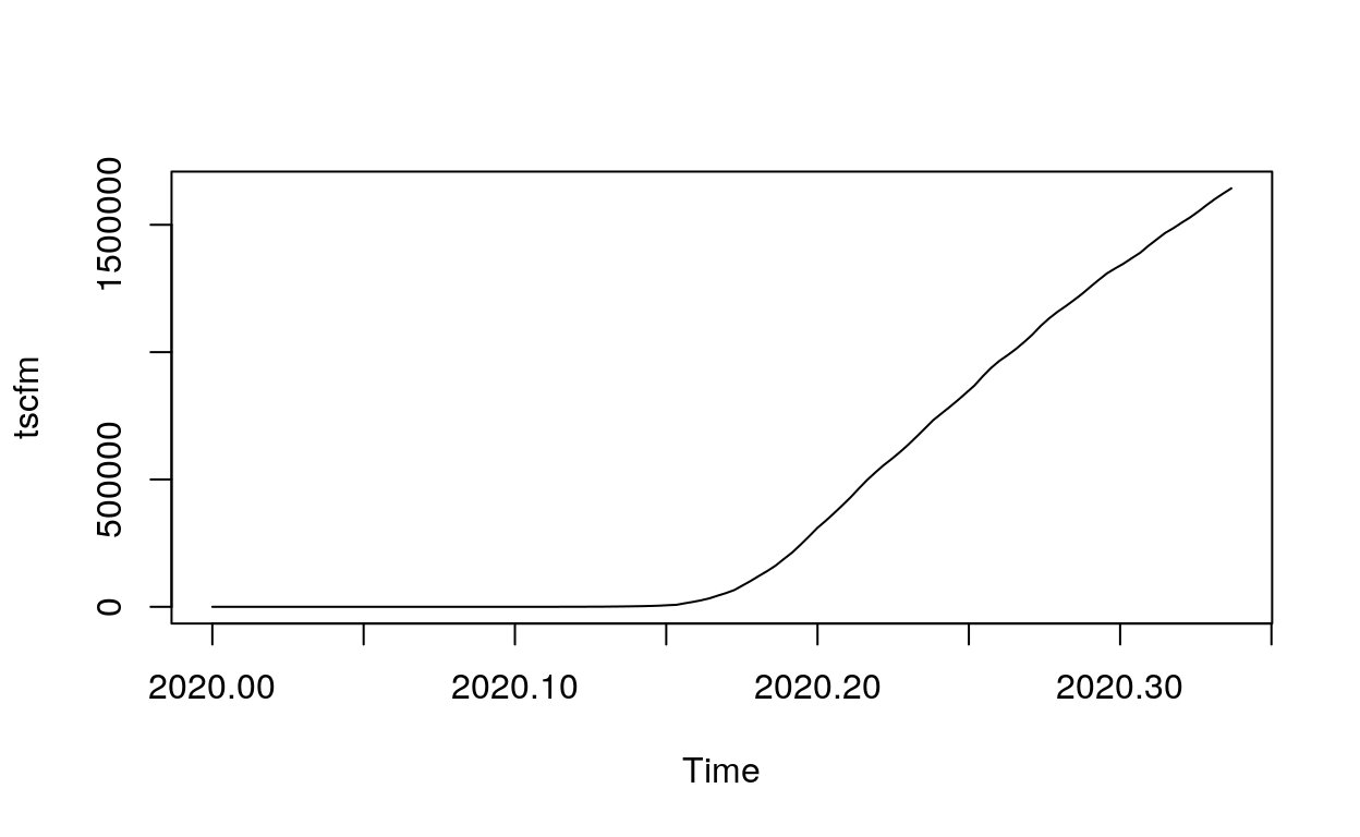
As we can see from the plot, take the death case of US for instance, the number of deaths began to increase significantly around the 25th day.
Then we can feed them into ARIMA (Autoregressive Moving Average Model) models:
#TS analysis with auto.arima founction
arc <- auto.arima(tscfm)
summary(arc)
Series: tscfm
ARIMA(2,2,2)

Coefficients:
         ar1      ar2      ma1     ma2
      1.2494  -0.9336  -1.4171  0.9170
s.e.  0.0319   0.0362   0.0740  0.0434

sigma^2 estimated as 3582037:  log likelihood=-1093.01
AIC=2196.02   AICc=2196.54   BIC=2210.04

Training set error measures:
                   ME    RMSE      MAE      MPE     MAPE MASE
Training set 242.3179 1846.27 1087.874 1.831374 6.710824  NaN
                    ACF1
Training set -0.08393917
By summarizing the model, we learn that the error rate (MAPE: Mean absolute percentage error) is 9.489553, which is not too bad. And the ARIMA model here is ARIMA(1, 2, 1).
ARIMA (p, d, q):
- p: Represents the lags of the time series data itself used in the prediction model, also called the AR/Auto-Regressive term.
- d: Represents the time series data that needs to be differentialized by several orders of magnitude to be stable, also called the integrated term.
- q: Represents the lagged number (lags) of prediction errors used in the prediction model, also called the MA/Moving Average term.
So here the ARIMA (1, 2, 1) model means: The level of the process, measured as the most resent value, plus a trend measured as the most recent change in the process.
More specifically: d = 2, adaptive trend in addition on the level.
Step 4: Prediction
Use the current model to do prediction for the next week (7 days).
fc1 <- forecast(arc, h=7) #predict for next 7 days
summary(fc1)
Forecast method: ARIMA(2,2,2)

Model Information:
Series: tscfm
ARIMA(2,2,2)

Coefficients:
         ar1      ar2      ma1     ma2
      1.2494  -0.9336  -1.4171  0.9170
s.e.  0.0319   0.0362   0.0740  0.0434

sigma^2 estimated as 3582037:  log likelihood=-1093.01
AIC=2196.02   AICc=2196.54   BIC=2210.04

Error measures:
                   ME    RMSE      MAE      MPE     MAPE MASE
Training set 242.3179 1846.27 1087.874 1.831374 6.710824  NaN
                    ACF1
Training set -0.08393917

Forecasts:
          Point Forecast   Lo 80   Hi 80   Lo 95   Hi 95
2020.3395        1663851 1661426 1666277 1660142 1667561
2020.3422        1685352 1680289 1690415 1677609 1693095
2020.3450        1707999 1700213 1715784 1696092 1719905
2020.3477        1731241 1720719 1741763 1715148 1747334
2020.3504        1754158 1740710 1767605 1733591 1774724
2020.3532        1776111 1759283 1792940 1750375 1801848
2020.3559        1797166 1776323 1818009 1765290 1829043
plot(fc1)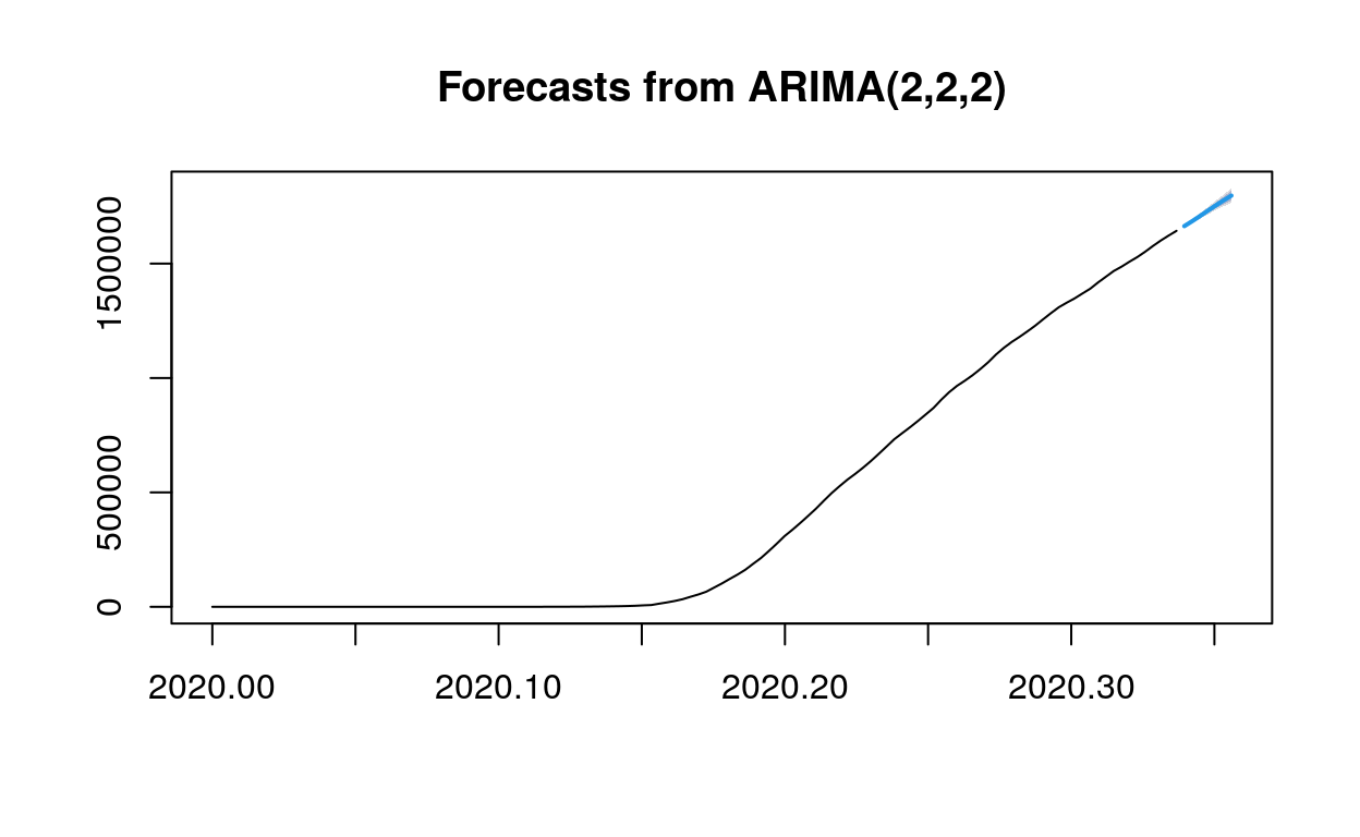
As we can see from the forecast matrix, on day one, there is a 95% probability that the predicted value will be between 761934.4 and 768048.2, and an 80% probability that the predicted value will be between 762992.5 and 766990.1…
Step 5: Residual analysis
#Residual analysis
acf(fc1$residuals)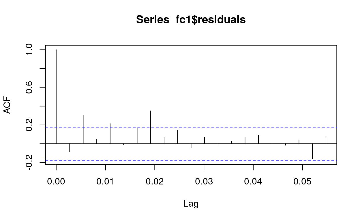
pacf(fc1$residuals)
plot(fc1$residuals)
qqnorm(fc1$residuals)
And we repeat the exact same process but for the confirmed deaths this time.
##time series analysis for confirmed deaths
tsdeath <- ts(countrydata$deaths, frequency = 365, start=c(2020,22), end=c(2020,92))
plot(tsdeath)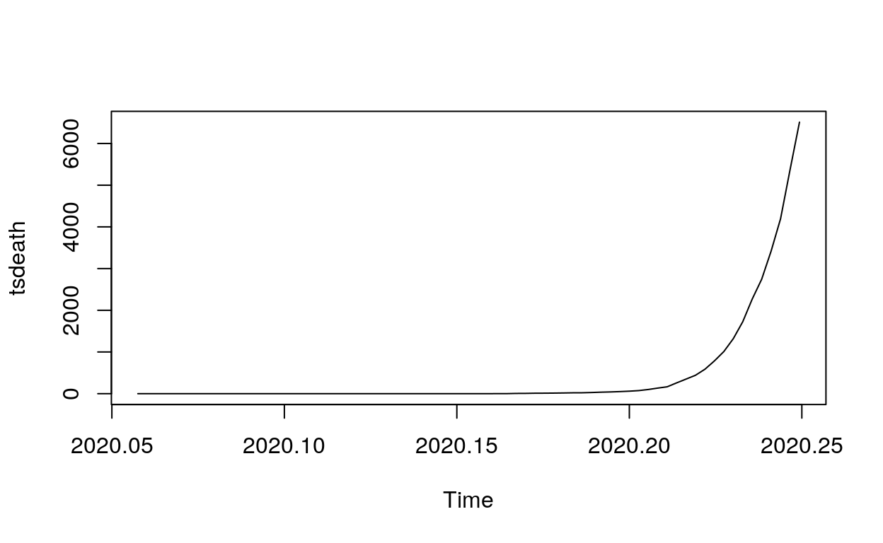
ard <- auto.arima(tsdeath)
summary(ard)
Series: tsdeath
ARIMA(0,2,0)

sigma^2 estimated as 3735:  log likelihood=-381.69
AIC=765.38   AICc=765.44   BIC=767.61

Training set error measures:
                   ME     RMSE      MAE      MPE     MAPE MASE
Training set 16.11268 60.25065 19.32394 4.638444 17.12991  NaN
                  ACF1
Training set 0.1439591
fc2 <- forecast(ard, h=7) #predict for next 7 days
summary(fc1)
Forecast method: ARIMA(2,2,2)

Model Information:
Series: tscfm
ARIMA(2,2,2)

Coefficients:
         ar1      ar2      ma1     ma2
      1.2494  -0.9336  -1.4171  0.9170
s.e.  0.0319   0.0362   0.0740  0.0434

sigma^2 estimated as 3582037:  log likelihood=-1093.01
AIC=2196.02   AICc=2196.54   BIC=2210.04

Error measures:
                   ME    RMSE      MAE      MPE     MAPE MASE
Training set 242.3179 1846.27 1087.874 1.831374 6.710824  NaN
                    ACF1
Training set -0.08393917

Forecasts:
          Point Forecast   Lo 80   Hi 80   Lo 95   Hi 95
2020.3395        1663851 1661426 1666277 1660142 1667561
2020.3422        1685352 1680289 1690415 1677609 1693095
2020.3450        1707999 1700213 1715784 1696092 1719905
2020.3477        1731241 1720719 1741763 1715148 1747334
2020.3504        1754158 1740710 1767605 1733591 1774724
2020.3532        1776111 1759283 1792940 1750375 1801848
2020.3559        1797166 1776323 1818009 1765290 1829043
plot(fc1)
#Residual analysis
acf(fc2$residuals)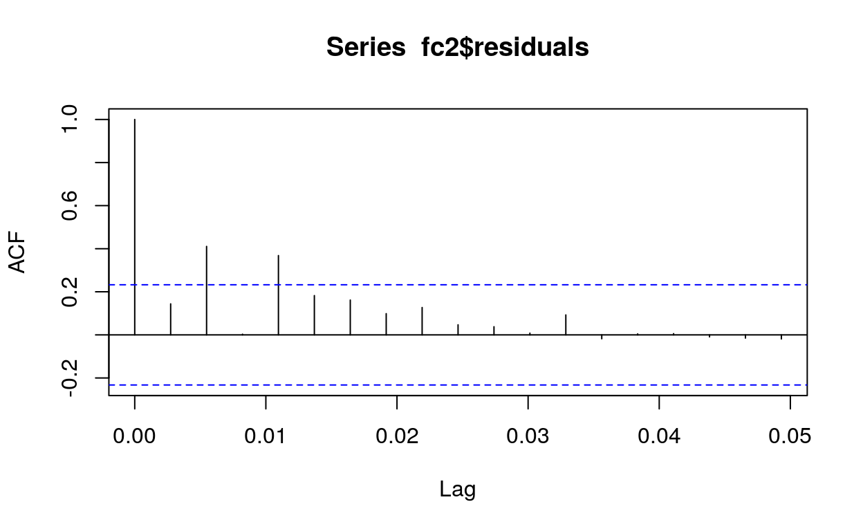
pacf(fc2$residuals)
plot(fc2$residuals)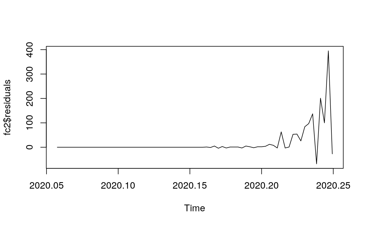
qqnorm(fc2$residuals)
tl;dr
# Load packages
library(tidyverse)
library(lubridate)
library(rvest)
library(stringdist)
library(forecast)

# Function to read the raw CSV files
# Files are aggregated to the country level and then converted to long format.
clean_jhd_to_long <- function(df) {
  df_str <- deparse(substitute(df))
  var_str <- substr(df_str, 1, str_length(df_str) - 4)

  df %>% group_by(`Country/Region`) %>%
    filter(`Country/Region` != "Cruise Ship") %>%
    select(-`Province/State`, -Lat, -Long) %>%
    mutate_at(vars(-group_cols()), sum) %>%
    distinct() %>%
    ungroup() %>%
    rename(country = `Country/Region`) %>%
    pivot_longer(
      -country,
      names_to = "date_str",
      values_to = var_str
    ) %>%
    mutate(date = mdy(date_str)) %>%
    select(country, date, !! sym(var_str))
}

confirmed_raw <- read_csv("https://raw.githubusercontent.com/CSSEGISandData/COVID-19/master/csse_covid_19_data/csse_covid_19_time_series/time_series_covid19_confirmed_global.csv")
deaths_raw <- read_csv("https://raw.githubusercontent.com/CSSEGISandData/COVID-19/master/csse_covid_19_data/csse_covid_19_time_series/time_series_covid19_deaths_global.csv")

jh_covid19_data <- clean_jhd_to_long(confirmed_raw) %>%
  full_join(clean_jhd_to_long(deaths_raw))

#select a country to do time series analysis with ARIMA model
slctcountry = "US" #This varible defines the county
countrydata <- subset(jh_covid19_data, country == slctcountry)

#time series analysis for confirmed cases
tscfm <- ts(countrydata$confirmed, frequency = 365.25, start=c(2020,1,22))
plot.ts(tscfm)

#TS analysis with auto.arima founction
arc <- auto.arima(tscfm)
summary(arc)

fc1 <- forecast(arc, h=7) #predict for next 7 days
summary(fc1)
plot(fc1)

#Residual analysis
acf(fc1$residuals)

pacf(fc1$residuals)

plot(fc1$residuals)

qqnorm(fc1$residuals)

##time series analysis for confirmed deaths
tsdeath <- ts(countrydata$deaths, frequency = 365, start=c(2020,22), end=c(2020,92))
plot(tsdeath)

ard <- auto.arima(tsdeath)
summary(ard)

fc2 <- forecast(ard, h=7) #predict for next 7 days
summary(fc1)
plot(fc1)

#Residual analysis
acf(fc2$residuals)

pacf(fc2$residuals)

plot(fc2$residuals)

qqnorm(fc2$residuals)
To go further with our pedagogical platform
- Our Coding School
- Our Potential Modules
- Module 1: Data Visualizations
- Module 2: Data Warehouse
- Module 3: News Collection and Analysis
- Module 4: Predictive Modelling
- Module 5: Social Media Collection and Analysis
- Module 6: Mapping
- Module 7: Bibliometrics
- Module 8: Topic Modelling
- Module 9: Covid-19 and International Flows
- Module 10: Covid-19 and Finance
- Module 11: Covid-19 and Public Policies
- Module 12: Covid-19 and Ethics
- Our Databases and APIs