Table of Contents
Pedagogical Material
As part of the Hacking Health Covid-19, the SKEMA Global Lab in AI provided to SKEMA’ students a fully developped data science environment to realize their project. See [here].
For this specific module, this team used these following courses:
- Module 1: Data Visualizations
- Module 2: Data Warehouse
- Module 6: Mapping
- Module 11: Covid-19 and Public Policies
- Module 12: Covid-19 and Ethics
Project Presentation
The goal of the project is to retrieve data from different databases and analyse it to find out if correlation can be found between the political regime and the number of deaths from the SARS-CoV-2 commonly named covid-19.
Technical Process
Collecting Data
Democracy Index
First we start by retrieving democracy index from Sherbrooke University (EIU.DEMO.GLOBAL, 2017, 163 Countries).
#Retrieving DEMOCRACY INDEX from Sherbrooke University (EIU.DEMO.GLOBAL, 2017, 163 Countries)

Democracy.Index =c( 2.55, 7.24, 5.98, 3.56, 8.61, 3.62, 1.93, 6.96, 4.11, 9.09, 8.42, 2.65, 2.71, 5.43,
                    3.13, 7.78, 5.61, 5.08, 5.49, 4.87, 7.81, 6.86, 7.03, 4.75, 2.33, 3.63, 3.61, 9.15,
                    7.88, 1.52, 7.84, 3.1, 7.59, 6.67, 3.71, 3.25, 1.61, 1.08, 8, 7.88, 3.93, 6.63, 3.31,
                    9.22, 2.76, 6.66, 3.36, 2.69, 6.02, 2.37, 8.08, 7.79, 3.03, 7.98, 3.42, 9.03, 7.8, 3.61,
                    4.06, 5.93, 6.69, 7.29, 5.86, 3.14, 1.81, 1.98, 6.46, 4.03, 5.72, 6.64, 7.23, 6.39, 4.09,
                    2.45, 9.15, 9.58, 7.79, 7.98, 7.29, 7.88, 3.87, 3.06, 5.11, 5.11, 3.85, 2.37, 6.64, 7.25,
                    4.72, 5.23, 2.32, 7.41, 8.81, 5.57, 5.11, 6.54, 5.49, 5.64, 4.87, 8.22, 3.82, 6.41, 5.94,
                    6.5, 5.69, 4.02, 3.83, 6.31, 5.18, 4.66, 3.76, 4.44, 9.87, 9.26, 3.04, 5.09, 1.95, 4.26,
                    7.08, 6.03, 6.31, 8.89, 6.49, 6.71, 6.67, 7.84, 3.19, 6.44, 8.53, 3.17, 3.19, 6.43, 6.15,
                    6.41, 4.66, 6.32, 7.16, 7.5, 2.15, 6.48, 9.39, 9.03, 6.76, 1.43, 1.93, 7.73, 5.47, 1.5,
                    7.62, 4.63, 7.19, 3.05, 7.04, 6.32, 1.72, 4.88, 5.69, 8.12, 3.87, 3.08, 2.07, 5.68, 3.16)

# Retrieving ISO COUNTRY CODE from Sherbrooke University

ISO = c("AFG", "ZAF", "ALB", "DZA", "DEU", "AGO", "SAU", "ARG", "ARM", "AUS", "AUT", "AZE", "BHR", "BGD", "BLR",
        "BEL", "BEN", "BTN", "BOL", "BIH", "BWA", "BRA", "BGR", "BFA", "BDI", "KHM", "CMR", "CAN", "CPV", "CAF",
        "CHL", "CHN", "CYP", "COL", "COM", "COG", "COD", "PRK", "KOR", "CRI", "CIV", "HRV", "CUB", "DNK", "DJI",
        "DOM", "EGY", "ARE", "ECU", "ERI", "ESP", "EST", "SWZ", "USA", "ETH", "FIN", "FRA", "GAB", "GMB", "GEO",
        "GHA", "GRC", "GTM", "GIN", "GNQ", "GNB", "GUY", "HTI", "HND", "HUN", "IND", "IDN", "IRQ", "IRN", "IRL",
        "ISL", "ISR", "ITA", "JAM", "JPN", "JOR", "KAZ", "KEN", "KGZ", "KWT", "LAO", "LSO", "LVA", "LBN", "LBR",
        "LBY", "LTU", "LUX", "MKD", "MDG", "MYS", "MWI", "MLI", "MAR", "MUS", "MRT", "MEX", "MDA", "MNG", "MON",
        "MOZ", "MMR", "NAM", "NPL", "NIC", "NER", "NGA", "NOR", "NZL", "OMN", "UGA", "UZB", "PAK", "PAN", "PNG",
        "PRY", "NLD", "PER", "PHL", "POL", "PRT", "QAT", "ROM", "GBR", "RUS", "RWA", "SLV", "SEN", "YUG", "SLE",
        "SGP", "SVK", "SVN", "SDN", "LKA", "SWE", "CHE", "SUR", "SYR", "TJK", "TWN", "TZA", "TCD", "CZE", "THA",
        "TMP", "TGO", "TTO", "TUN", "TKM", "TUR", "UKR", "URY", "VEN", "VNM", "YEM", "ZMB", "ZWE")
# Creation of a dataframe called 'democracy'
democracy = data.frame(ISO,Democracy.Index)

# Ordering democracy dataframe by alphabetical order on iso country code
democracy <- democracy[order(ISO),]
#Writing of the democracy index excel file
library(writexl)
write_xlsx(x = democracy, path = "Datasets/dataset_democracy_index.xlsx", col_names = TRUE)
Press Liberty Index
We continue by retrieving the press liberty index from Sherbrook University (PF.LIB.PRESS.RSF.IN, 2017, 166 Countries).
#Retrieving PRESS LIBERTY INDEX from Sherbrooke University (PF.LIB.PRESS.RSF.IN, 2017, 166 Countries)

PRESS.LIBERTY.INDEX =c( 39.46, 20.12, 29.92, 42.83, 14.97, 40.42, 66.02, 25.07, 30.38, 16.02, 13.47, 56.4, 58.88,
                        48.36, 52.43, 12.75, 30.32, 30.73, 33.88, 27.83, 24.93, 33.58, 35.01, 23.85, 55.78, 42.07,
                        41.59, 16.53, 18.02, 36.12, 20.53, 77.66, 19.79, 41.47, 24.33, 36.73, 52.67, 84.98, 27.61,
                        11.93, 30.42, 29.59, 71.75, 10.36, 70.54, 26.76, 55.78, 39.39, 33.64, 84.24, 18.69, 13.55,
                        51.27, 23.88, 50.34, 8.92, 22.24, 34.83, 46.7, 27.76, 17.95, 30.89, 39.33, 33.15, 66.47,
                        30.09, 26.8, 26.36, 43.75, 29.01, 42.94, 39.93, 54.03, 65.12, 14.08, 13.03, 31.01, 26.26,
                        12.73, 29.44, 43.24, 54.01, 31.2, 30.92, 30.45, 33.61, 66.41, 28.78, 18.62, 33.01, 31.12,
                        56.81, 21.37, 14.72, 35.74, 26.71, 46.89, 28.97, 38.27, 42.42, 26.67, 26.49, 48.97, 30.41,
                        28.95, 33.65, 31.05, 41.82, 17.08, 33.02, 31.01, 27.21, 39.69, 7.6, 13.98, 40.46, 35.94, 66.11,
                        43.55, 32.12, 25.07, 35.64, 11.28, 30.98, 41.08, 26.47, 15.77, 39.83, 24.46, 22.26, 49.45, 54.11,
                        27.24, 26.72, 28.05, 30.73, 51.1, 15.51, 21.7, 65.95, 73.56, 48.16, 44.34, 8.27, 12.13, 16.07,
                        81.49, 50.27, 24.37, 30.65, 39.66, 16.91, 44.69, 32.82, 30.75, 20.62, 32.22, 84.19, 52.98, 33.19,
                        17.43, 42.94, 73.96, 65.8, 36.48, 41.44)

#Retrieving ISO COUNTRY CODE from Sherbrooke University

ISO = c("AFG", "ZAF", "ALB", "DZA", "DEU", "AGO", "SAU", "ARG", "ARM", "AUS", "AUT", "AZE", "BHR", "BGD", "BLR", "BEL",
        "BEN", "BTN", "BOL", "BIH", "BWA", "BRA", "BGR", "BFA", "BDI", "KHM", "CMR", "CAN", "CPV", "CAF", "CHL", "CHN",
        "CYP", "COL", "COM", "COG", "COD", "PRK", "KOR", "CRI", "CIV", "HRV", "CUB", "DNK", "DJI", "DOM", "EGY", "ARE",
        "ECU", "ERI", "ESP", "EST", "SWZ", "USA", "ETH", "FIN", "FRA", "GAB", "GMB", "GEO", "GHA", "GRC", "GTM", "GIN",
        "GNQ", "GNB", "GUY", "HTI", "HND", "HUN", "IND", "IDN", "IRQ", "IRN", "IRL", "ISL", "ISR", "ITA", "JAM", "JPN",
        "JOR", "KAZ", "KEN", "KGZ", "KSV", "KWT", "LAO", "LSO", "LVA", "LBN", "LBR", "LBY", "LTU", "LUX", "MKD", "MDG",
        "MYS", "MWI", "MLI", "MAR", "MUS", "MRT", "MEX", "MDA", "MNG", "MON", "MOZ", "MMR", "NAM", "NPL", "NIC", "NER",
        "NGA", "NOR", "NZL", "OMN", "UGA", "UZB", "PAK", "PAN", "PNG", "PRY", "NLD", "PER", "PHL", "POL", "PRT", "QAT",
        "ROM", "GBR", "RUS", "RWA", "SLV", "SEN", "YUG", "SLE", "SGP", "SVK", "SVN", "SOM", "SDN", "SSD", "LKA", "SWE",
        "CHE", "SUR", "SYR", "TJK", "TWN", "TZA", "TCD", "CZE", "THA", "TMP", "TGO", "TTO", "TUN", "TKM", "TUR", "UKR",
        "URY", "VEN", "VNM", "YEM", "ZMB", "ZWE")
#Creation of a DATAFRAME called PRESS
press = data.frame(ISO,PRESS.LIBERTY.INDEX)

#Ordering PRESS DATAFRAME by alphabetical order on ISO COUNTRY CODE
press <- press[order(ISO),]

#TRANSFORMING the REPRESSION PRESS INDEX into a LIBERTY PRESS INDEX
press$Press.Liberty.Index <- 100 - press$PRESS.LIBERTY.INDEX

#DELETING the old REPRESSION COLUMN
press$PRESS.LIBERTY.INDEX <- NULL
#Writing of the PRESS LIBERTY INDEX EXCEL FILE
library(writexl)
write_xlsx(x = press, path = "Datasets/dataset_press_liberty_index.xlsx", col_names = TRUE)
Covid 19 Cases
Then we retrieve covid-19 cases from the European Union Open Data Portal (Covid 19 cases, 28-04-2020, — Countries).
library(readr)

# Downloading data from the Data Europa Portal and saving xlsx file into covid19_cases variable
covid19_cases <- read_csv("https://opendata.ecdc.europa.eu/covid19/casedistribution/csv")

#Deleting unwanted columns
covid19_cases[,1] <- NULL
covid19_cases[,7] <- NULL
covid19_cases[,9] <- NULL

#Renaming columns
names(covid19_cases)[1] <- "Day"
names(covid19_cases)[2] <- "Month"
names(covid19_cases)[3] <- "Year"
names(covid19_cases)[4] <- "Cases"
names(covid19_cases)[5] <- "Deaths"
names(covid19_cases)[6] <- "Country"
names(covid19_cases)[7] <- "ISO"
names(covid19_cases)[8] <- "Population"

head(covid19_cases)
# A tibble: 6 x 8
    Day Month  Year Cases Deaths Country     ISO   Population
  <dbl> <dbl> <dbl> <dbl>  <dbl> <chr>       <chr>      <dbl>
1    26     5  2020   591      1 Afghanistan AFG     37172386
2    25     5  2020   584      2 Afghanistan AFG     37172386
3    26     5  2020     0      0 Aruba       ABW       105845
4    25     5  2020     0      0 Aruba       ABW       105845
5    26     5  2020     6      0 Albania     ALB      2866376
6    25     5  2020     9      1 Albania     ALB      2866376
# Writing of the DATASET EXCEL FILE

library(writexl)
write_xlsx(x = covid19_cases, path = "Datasets/dataset_covid19_cases_index.xlsx", col_names = TRUE)
Per Capita Income Index
We continue by retrieving the Per Capita Income from the World Bank (NY.GNP.PCAP.CD, 2018, 229 Countries).
library(WDI)
library(plyr)

#RETRIEVING of the RNB PER INHABITANT for ALL COUNTRIES
RNB_hab_year <- WDI(indicator = "NY.GNP.PCAP.CD",
                   country = "all",
                   start = 2018,
                   end = NULL)


#Handling MISSING VALUES
RNB_hab_year <- na.omit(RNB_hab_year)

#RENAMING of COLUMNS
names(RNB_hab_year)[1] <- "ISO2"
names(RNB_hab_year)[2] <- "Country"
names(RNB_hab_year)[3] <- "RNB.Inhab.Year"


#DELETING UNWANTED COLMUNS
RNB_hab_year$year <- NULL
RNB_hab_year[2] <- NULL
We load voice accountability index, corruption index, rule of law index and govnerment effectiveness index from the World Governance Indicators data base of the World Bank (2018).
library(readxl)
library(dplyr)

#LOADING WGI dataset VOICE ACCOUNTABILITY
dataset_WGI1 <- read_excel("Datasets/World Governance Indicator/dataset_WGI_2018_Voice_Accountability.xlsx")

#DELETING specific ROWS where values == #N/A

dataset_WGI1 <- subset(dataset_WGI1, Estimate != "#N/A")

#DELETING UNWANTED COLUMNS
dataset_WGI1 <- dataset_WGI1[1:3]

#RENAMING COLUMNS
names(dataset_WGI1)[1] <- "Country"
names(dataset_WGI1)[2] <- "ISO"
names(dataset_WGI1)[3] <- "Voice Accountability"


#################################################################
#LOADING WGI dataset CORRUPTION
dataset_WGI2 <- read_excel("Datasets/World Governance Indicator/dataset_WGI_2018_Corruption.xlsx")

#DELETING specific ROWS where values == #N/A
dataset_WGI2 <- subset(dataset_WGI2, Estimate != "#N/A")

#DELETING UNWANTED COLUMNS
dataset_WGI2 <- dataset_WGI2[1:3]

#RENAMING COLUMNS
names(dataset_WGI2)[1] <- "Country"
names(dataset_WGI2)[2] <- "ISO"
names(dataset_WGI2)[3] <- "Corruption"

#################################################################
#LOADING WGI dataset RULE OF LAW
dataset_WGI3 <- read_excel("Datasets/World Governance Indicator/dataset_WGI_2018_Rule_of_Law.xlsx")

#DELETING specific ROWS where values == #N/A
dataset_WGI3 <- subset(dataset_WGI3, Estimate != "#N/A")

#DELETING UNWANTED COLUMNS
dataset_WGI3 <- dataset_WGI3[1:3]

#RENAMING COLUMNS
names(dataset_WGI3)[1] <- "Country"
names(dataset_WGI3)[2] <- "ISO"
names(dataset_WGI3)[3] <- "Rule of Law"

#################################################################
#LOADING WGI dataset GOVERNMENT EFFECTIVENESS
dataset_WGI4 <- read_excel("Datasets/World Governance Indicator/dataset_WGI_2018_Government_Effectiveness.xlsx")

#DELETING specific ROWS where values == #N/A
dataset_WGI4 <- subset(dataset_WGI4, Estimate != "#N/A")

#DELETING UNWANTED COLUMNS
dataset_WGI4 <- dataset_WGI4[1:3]

#RENAMING COLUMNS
names(dataset_WGI4)[1] <- "Country"
names(dataset_WGI4)[2] <- "ISO"
names(dataset_WGI4)[3] <- "Government Effectiveness"
Universal Health Coverage Index
Finally we load the Universal Health Coverage (UHC) - Service Capacity and Acess index from the World Health Organization (2018).
library(readxl)
library(dplyr)

#IMPORT and SAVING of ISO COUNTRY CODE index
service_capacity_access <- read_excel("Datasets/UHC-service_capacity_access.xlsx")
Data Wrangling
Merging the press liberty index with the democracy index.
#MERGING the PRESS LIBERTY INDEX with the DEMOCRACY INDEX (different rows in ISO CODE)
dataset_intermediaire_clustering = merge(press, democracy, by="ISO")
Creation of a translation index for ISO country code and country name.
library(readxl)
library(dplyr)

#IMPORT and SAVING of ISO COUNTRY CODE index
ISO_COUNTRY_REDUCED <- read_excel("Datasets/ISO_COUNTRY_TRANSLATION_V2.xlsx")

ISO_COUNTRY_REDUCED <- filter(ISO_COUNTRY_REDUCED, ISO_COUNTRY_REDUCED$ISO != "N/A")
Saving of the iso_country_reduced index in a dataset excel file.
#Writing of the DATASET EXCEL FILE
library(writexl)

write_xlsx(x = ISO_COUNTRY_REDUCED, path = "Datasets/iso_country_reduced.xlsx", col_names = TRUE)
Filtering and summarizing of Death cases and Confirmed cases within the dataset final excel file.
library(dplyr)

#FILTERING DEATHS CASES in the covid19_cases sum up file
sum_deaths_country <- covid19_cases %>%
  group_by(ISO) %>%
  summarize(Deaths.Cases = sum(Deaths, na.rm=TRUE))


#FILTERING CONFIRMED CASES in the covid19_cases sum up file
sum_confirmed_country <- covid19_cases %>%
  group_by(ISO) %>%
  summarize(Confirmed.Cases = sum(Cases, na.rm=TRUE))


#FILTERING POPULATION in the covid19_cases sum up file
 population_country <- covid19_cases %>%
  group_by(ISO) %>%
  summarize(Population = mean(Population, na.rm=TRUE))
Merging death cases sum, confirmed cases sum and country’s population in the dataset final file.
library(dplyr)

#LOADINF of the ISO COUNTRY CODE into DATASET INTERMEDIAIRE COVID
dataset_intermediaire_covid <- ISO_COUNTRY_REDUCED

#MERGING DEATH CASES SUM and DATASET INTERMEDIAIRE COVID by ISO code
dataset_intermediaire_covid = merge(sum_deaths_country, dataset_intermediaire_covid, by = "ISO")

#MERGING CONFIRMED CASES SUM and DATASET INTERMEDIAIRE COVID by ISO code
dataset_intermediaire_covid = merge(sum_confirmed_country, dataset_intermediaire_covid, by = "ISO")

#MERGING POPULATION COUNTRY SUM and DATASET INTERMEDIAIRE COVID by ISO code
dataset_intermediaire_covid = merge(population_country, dataset_intermediaire_covid, by = "ISO")
#MOVING COLUMNS in order to have COUNTRY'S NAME as FIRST COLUMN
dataset_intermediaire_covid <- dataset_intermediaire_covid[, c(1, 5, 6, 2, 3, 4)]
Calculation of Deaths ratio and confirmed cases among the total population, deaths ratio among confirmed cases.
dataset_intermediaire_covid$Death.Ratio.Population <- (dataset_intermediaire_covid$Deaths.Cases
                                                       / dataset_intermediaire_covid$Population) * 1000000
dataset_intermediaire_covid$Confirmed.Ratio.Population <- (dataset_intermediaire_covid$Confirmed.Cases
                                                           / dataset_intermediaire_covid$Population) * 1000000
dataset_intermediaire_covid$Death.Ratio.Confirmed <- (dataset_intermediaire_covid$Deaths.Cases
                                                      / dataset_intermediaire_covid$Confirmed.Cases) * 100
Saving data in a dataset excel file.
dataset_final_covid <- dataset_intermediaire_covid

#Writing of the DATASET EXCEL FILE
library(writexl)

write_xlsx(x = dataset_final_covid, path = "Datasets/dataset_final_covid.xlsx", col_names = TRUE)
Merging the intermediary clustering dataset with the per capita income by year.
library(dplyr)

#INNER_JOIN the RNB PER INHABITANT with the DATASET FINAL (different rows in ISO CODE)
dataset_intermediaire_clustering = inner_join(dataset_intermediaire_covid, RNB_hab_year, by = "ISO2")
dataset_intermediaire_clustering = inner_join(dataset_intermediaire_clustering, press, by = "ISO")
dataset_intermediaire_clustering = inner_join(dataset_intermediaire_clustering, democracy, by = "ISO")

#DELETING UNWANTED COLUMNS
dataset_intermediaire_clustering[3:9] <- NULL
Merging of voice accountability index, corruption index, rule of law index and govnerment effectiveness index together.
#MERGING VOICE ACCOUNTABILITY and CORRUPTION by ISO code
dataset_WGI2$Country  <- NULL
dataset_intermediaire_WGI = merge(dataset_WGI1, dataset_WGI2, by = "ISO")

#MERGING VOICE ACCOUNTABILITY, CORRUPTION and RULE of LAW by ISO code
dataset_WGI3$Country  <- NULL
dataset_intermediaire_WGI = merge(dataset_intermediaire_WGI, dataset_WGI3, by = "ISO")

#MERGING VOICE ACCOUNTABILITY, CORRUPTION, RULE of LAW and GOVERNMENT EFFECTIVENESS by ISO code
dataset_WGI4$Country  <- NULL
dataset_intermediaire_WGI = merge(dataset_intermediaire_WGI, dataset_WGI4, by = "ISO")

#MERGING VOICE ACCOUNTABILITY, CORRUPTION, RULE of LAW and GOVERNMENT EFFECTIVENESS by ISO code
dataset_intermediaire_WGI$Country  <- NULL
dataset_intermediaire_clustering = merge(dataset_intermediaire_clustering, dataset_intermediaire_WGI, by = "ISO")
Combining of ISO country code translation file and Universal Health Coverage (UHC) - Service Capacity and Acess index.
library(dplyr)

#TESTING differences existance
dataset_antijoin = anti_join(service_capacity_access, ISO_COUNTRY_REDUCED, by = "Country")

#JOINING SERVICE CAPACITY and ACCESS with ISO COUNTRY file
service_capacity_access_index = full_join(service_capacity_access, ISO_COUNTRY_REDUCED, by = "Country")

service_capacity_access_index <- na.omit(service_capacity_access_index)

names(service_capacity_access_index)[2] <- "Service Capacity and Access"

#SAVING and WRITING of the DATASET EXCEL FILE
library(writexl)

write_xlsx(x = service_capacity_access_index, path = "Datasets/service_capacity_access_index.xlsx", col_names = TRUE)
Merging dataset final and service capacity and access index.
#MERGING DATASET INTERMEDIAIRE CLUSTERING and SERVICE CAPACITY ACCESS INDEX by ISO code
service_capacity_access_index$Country  <- NULL
dataset_final_clustering = merge(dataset_intermediaire_clustering, service_capacity_access_index, by = "ISO")
dataset_final_clustering$ISO2 <- NULL
Saving dataset World Governance Indicator plus Access and Capacity to the Health Care system in a excel file.
#SAVING DATASET FINAL in a EXCEL FILE
write_xlsx(x = dataset_final_clustering, path = "Datasets/dataset_final_WGI_capacity_access.xlsx", col_names = TRUE)
Saving dataset final in a excel file.
#SAVING DATASET FINAL in a EXCEL FILE
write_xlsx(x = dataset_final_clustering, path = "Datasets/dataset_intermediaire_clustering.xlsx", col_names = TRUE)
Data Analysis
Now that we’ve got our final dataset regrouping, for 196 countries, informations about the covid-19 such as : Comfired cases number, Death cases number and ratio like dead person among confirmed person, confirmed cases among total population, Death cases among total population but also the total population of the country and their ISO code and names. We decided to run a correlation test to find patterns that could be interesting and to complete this test by a p-value test. We want to confirm if correlation found are real one, in other words that those correlations are significant or not. To run this final test, the p-value chosen was 0.05.
Correlation tests and p-value analysis
library(corrplot)

#LOADIND and SAVING of DATASET FINAL
dataset_intermediaire_covid_correl <- select(dataset_final_covid, 'Population', 'Confirmed.Cases',
                                             'Deaths.Cases', 'Death.Ratio.Population',
                                             'Confirmed.Ratio.Population', 'Death.Ratio.Confirmed')


#COMPUTATION of the CENTERING MATRIX
mcov <- scale(dataset_intermediaire_covid_correl)

mcov <- na.omit(mcov)

#SAVING MCOV as a DATA FRAME
covariance_matrix <- as.data.frame(mcov)


#CORRELATION TEST with HANDLING of MISSING VALUES
mcor <- cor(covariance_matrix, method = "pearson", use = "complete.obs")

#SAVING MCOR as a DATA FRAME
correlation_matrix <- as.data.frame(mcor)

#DISPLAYING of CORRELATION GRAPHIC
col <- colorRampPalette(c("#BB4444", "#EE9988", "#FFFFFF", "#77AADD", "#4477AA"))

corrplot(mcor, method="color", col=col(200), type="upper", order="hclust",
         number.cex = .9, addCoef.col = "black", tl.col="black", tl.srt=45,
         insig = "blank", diag=TRUE )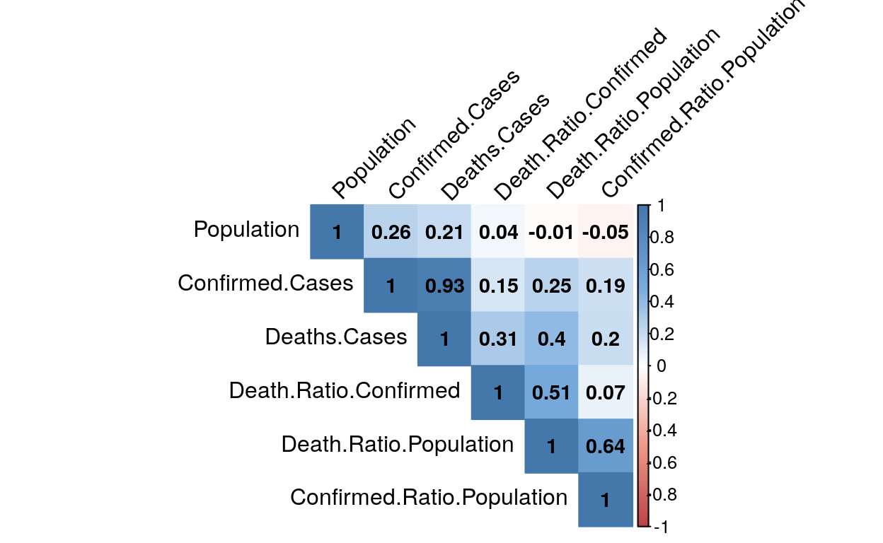
By performing this correlation test on the dataset regrouping figures about covid-19, we see that the correlation between deaths and confirmed cases related to covid-19 is strong. This is no surprise as every critical or dead patient needs to be tested as the World health Organisation recommended. Furthermore, there is a strong correlation between the number of deaths per inhabitant and the number of confirmed cases per inhabitant.
Others relations can be more surprising as the population and confirmed cases, or deaths cases, that are not related at all. This don’t come as a matter of facts as we can picture that the more your population is big as a country, the more cases you should have.
#COMPUTATION of the P-VALUE COEEFICIENT
library(Hmisc)
p_value <- rcorr(as.matrix(correlation_matrix))

p_value_matrix <- as.data.frame(p_value$P)


#DISPLAYING of SIGNIFICANT P-VALUE CORRELATION GRAPHIC
library(corrplot)

col <- colorRampPalette(c("#BB4444", "#EE9988", "#FFFFFF", "#77AADD", "#4477AA"))

corrplot(p_value$r, method="color", col=col(200), type="upper", order="hclust",
         number.cex = .9, addCoef.col = "black", tl.col="black", tl.srt=45,
         p.mat = p_value$P, sig.level = 0.05, insig = "blank", diag=TRUE )
After performing a correlation test with p-value to determine whether the correlations obtained are significant or not, the correlations that still exist appear different. Indeed, only the correlation between the number of confirmed cases and the number of deaths appears to be significant.
A surprising negative correlation appears between the size of the country’s population and its number of deaths relative to the population. Indeed, this correlation did not appear on the simple correlation test.
We perfom same test on our final dataset regrouping, for 147 countries, information about their revenues and governance style such as : Press Liberty index, Democracy index, Per Capita Income index, Corruption index, Rule of Law index, Government Effectiveness index, Voice and Accountability index and Service Capacity and Acces index. We decided to run a correlation test to find pattern that could be interesting and to complete this test by a p-value test to confirm if correlations found are significant or not. To run this final test, the p-value chosen is 0.05.
#LOADIND and SAVING of DATASET FINAL
dataset_intermediaire_clustering_correl <- select(dataset_final_clustering, 'RNB.Inhab.Year', 'Press.Liberty.Index',
                                                  'Democracy.Index', 'Voice Accountability', 'Corruption', 'Rule of Law',
                                                  'Government Effectiveness', 'Service Capacity and Access')

#COMPUTATION of the CENTERING MATRIX
mcov2 <- scale(dataset_intermediaire_clustering_correl)

mcov2 <- na.omit(mcov2)

#SAVING MCOV as a DATA FRAME
covariance_matrix2 <- as.data.frame(mcov2)

#CORRELATION TEST with HANDLING of MISSING VALUES
mcor2 <- cor(covariance_matrix2, method = "pearson", use = "complete.obs")

#SAVING MCOR as a DATA FRAME
correlation_matrix2 <- as.data.frame(mcor2)

#DISPLAYING of CORRELATION GRAPHIC
col <- colorRampPalette(c("#BB4444", "#EE9988", "#FFFFFF", "#77AADD", "#4477AA"))

corrplot(mcor2, method="color", col=col(200), type="full", order="hclust", number.cex = .9,
         addCoef.col = "black", tl.col="black", tl.srt=45, insig = "blank", diag=TRUE )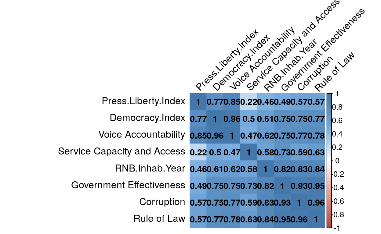
This first correlation matrix shows us correlations between variables. Every intersection between a line and a columns represent the correlation between those two variables. The more the blue is intense, the more the correlation is strong. Numbers in colored squares represent the correlation. If, and only if, this number is above 0.5 then the correlation can be interpreted as strong. Even if strong correlations can be found, this first matrix can’t tell us if those correlations are statistically confirmed, in other word that those correlations still exist after performing a p-value test on it.
We perform a p-value test to confirm or not correlations found.
#COMPUTATION of the P-VALUE COEEFICIENT
library(Hmisc)
p2_value <- rcorr(as.matrix(correlation_matrix2))

p_value_matrix2 <- as.data.frame(p2_value$P)

#DISPLAYING of SIGNIFICANT CORRELATION GRAPHIC
library(corrplot)

col <- colorRampPalette(c("#BB4444", "#EE9988", "#FFFFFF", "#77AADD", "#4477AA"))

corrplot(p2_value$r, method="color", col=col(200), type="full", order="hclust",
         number.cex = .9, addCoef.col = "black", tl.col="black", tl.srt=45,
         p.mat = p2_value$P, sig.level = 0.05, insig = "blank", diag=TRUE )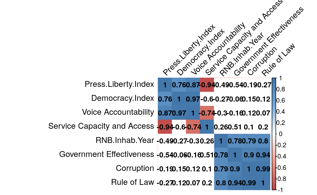
By doing this test, we clearly see that a lot of correlations precedently found, does not existe anymore. Every square still colored shows significant correlations. The blue ones a positive correlation, and red ones a negative one. By reading the matrix, we see that some indicators best decribe others, like the Rule of Law index which is strongly, and significantly, correlated to the RNB per Inhabitant per year, the Government effectiveness, the Corruption index. Therefore, if we only take it to perfom test, it will well represents the other ones.
Country segmentation by k-mean algorithm
After calculation of this correlation matrix under the p-value test, we decided to take only some of indicators to perfom a kmeans algorithm on a dataset of 147 countries.
Our goal is to create groups of country based on the evaluation of their : Service Capacity and Access index, Rule of law index and Voice Accountability index.
Before performing the kmeans algorithm, it is needed to by determine the optimal number of clusters. in order to avoid too vague clustering, it will be important not to fragment the dataset into more than 3 groups. By doing so, the subgroups should contain more than the 30 individuals needed to perform statistically reliable tests. Having 148 countries, the ideal groups would contain in the 45 to 50 countries.
The optimal number of clusters is determined prior to the execution of the kmeans agorithm. In order to determine this optimal number, the silhouette clustering test is performed.
For each observation, the silhouette coefficient corresponds to the difference between the average distance with observations from the same group (cohesion) and the average distance with observations from other neighbouring groups (separation). If this difference is negative, the observation is on average closer to the neighbouring group than to its own: it is therefore misclassified. Conversely, if this difference is positive, the point is on average closer to its group than to the neighbouring group: it is therefore well ranked.
#TEST SUR LES KMEANS

library(factoextra)
library(purrr)
library(cluster)

#LOADING of the DATASET FINAL2 into DATASET KMEANS1
dataset_kmeans_clustering_temps <- dataset_final_clustering

#Making the FIRST COLUMNS as ROWNAMES
dataset_kmeans_clustering <- dataset_kmeans_clustering_temps[,-1]
rownames(dataset_kmeans_clustering) <- dataset_kmeans_clustering_temps[,1]

#DELETING UNWANTED COLUMNS
dataset_kmeans_clustering <- select(dataset_kmeans_clustering, 'Voice Accountability',
                                    'Rule of Law', 'Service Capacity and Access')

#STANDARDIZATON of the DATASET KMEANS
scale(dataset_kmeans_clustering)

#LOOKING FOR the best number of CLUSTERS by SILHOUETTE method
set.seed(40)

fviz_nbclust(dataset_kmeans_clustering, k.max = 5, kmeans, method = "silhouette")
This silhouette clustering algorithm shows that 2 cluster is the optimal number. However, in order to avoid a too imprecise partitioning, the dataset will be subdivided into 3 groups which corresponds to the second optimal partitioning.
3 groups of countries will therefore be determined by the K-mean algorithm, but it is necessary to ensure the quality of the resulting clusters,to do a Gap Statistic test is performed. The Gap Statistic is a method developed by R. Tibshirani, G. Walther, and T. Hastie from the Standford University in 2001. they describe their method in the following way : “The technique uses the output of any clustering algorithm, comparing the change in within-cluster dispersion with that expected under an appropriate reference null distribution”. This means that the more the gap statistic number for each k is high, the better this number of clusters (k) represent a good clustering.
#CALCULATING the QUALITY of the CLUSTERING depending on NUMBERS of CLUSTERS
gap_stat <- clusGap(dataset_kmeans_clustering, FUN = kmeans,
                    nstart = 25, K.max = 5, B = 50)

#PRINT the RESULT
print(gap_stat, method = "firstmax")
Clustering Gap statistic ["clusGap"] from call:
clusGap(x = dataset_kmeans_clustering, FUNcluster = kmeans, K.max = 5,     B = 50, nstart = 25)
B=50 simulated reference sets, k = 1..5; spaceH0="scaledPCA"
 --> Number of clusters (method 'firstmax'): 2
         logW   E.logW         gap     SE.sim
[1,] 7.124733 6.991910 -0.13282300 0.03827945
[2,] 6.111907 6.300645  0.18873780 0.04121015
[3,] 5.770639 5.894331  0.12369158 0.03572097
[4,] 5.495059 5.617342  0.12228319 0.03330276
[5,] 5.313708 5.409056  0.09534801 0.03251540
fviz_gap_stat(gap_stat)
If 2 clusters still represents the optimal number of clusters, as the Silhouette method already indicated, 3 being the second best option, it is possible to choose 3 as the optimal number of clusters. This method is particularly sensitive to cluster overlapping which can explain why 3 is not the optimal number of clusters. Confirmation will be made by seeing groups of countries during the performation of the k-means algorithm. keeping in mind that 30 countries for each clusters is a minimum to perform statistics, 5 in the maximum number of clusters tested. Indeed, if 5 clusters are created they will contain less than 30 countries in each one and thus, statistical tests cannot be performed.
Once all the parameters of the k-mean algorithm have been determined, it should be applied to the dataset containing the variables selected for each country that are : : Voice Accoutability index, Rule of Law index and Service Capacity and Access index.
#APPLYING the KMEANS ALGORITHM
set.seed(2450)
clusters <- kmeans(dataset_kmeans_clustering, 3, nstart = 25)

fviz_cluster(clusters, data = dataset_kmeans_clustering)
#SAVING the COUNTRY'S CLUSTER NUMBER into DATASET FINAL2
dataset_kmeans_clustering$Cluster <- clusters$cluster
3 groups of 66, 32 and 50 countries sharing common characteristics according to the selected variables are obtained. As previously suspected, overlapping cluster can be observed which means that this clustering cannot be the best one. With that said, this overlapping is due to only 3 countries which does not represent a threat for the overhall clustering.
Saving dataset final in a excel file.
#SAVING DATASET FINAL in a EXCEL FILE
write_xlsx(x = dataset_kmeans_clustering, path = "Datasets/dataset_kmeans_clustering.xlsx", col_names = TRUE)
Covid-19 impact statistics by cluster
Once 3 clusters of countries have been obtained, analyses will be carried out to determine the impact of covid-19 on the countries belonging to the same cluster.
#Creation of CLUSTER 1 DATAFRAME
#RETRIEVING DATASET KMEANS CLUSTERING to add COUNTRY COLUMN
dataset_cluster_1_temp <- dataset_kmeans_clustering
dataset_cluster_1_temp$Country <- dataset_final_clustering$Country

#FILTERING only COUNTRIES in the CLUSTER 1
dataset_cluster_1 <- filter(dataset_cluster_1_temp, dataset_cluster_1_temp$Cluster == "1")

#MOVING COLUMNS in order to have COUNTRY'S NAME as FIRST COLUMN
dataset_cluster_1 <- dataset_cluster_1[, c(5, 1, 2, 3, 4)]
dataset_cluster_1 <- as.data.frame(dataset_cluster_1)

#SELECTION of COVID NUMBERS for countries in the CLUSTER 1 ONLY
dataset_covid_cluster_1 <- filter(dataset_final_covid, dataset_final_covid$Country %in% dataset_cluster_1$Country)

#COMPUTATION of MEANS for EACH COLUMNS
means_covid_cluster_1 <- colMeans(dataset_covid_cluster_1[4:9])
means_covid_cluster_1 <- as.data.frame(means_covid_cluster_1)

#DELETING ISO2 COLUMN
dataset_covid_cluster_1$ISO2 <- NULL


#RETRIEVING COVID INFORMATIONS by COUNTRY
dataset_covid_10_countries <- subset(dataset_covid_cluster_1, dataset_covid_cluster_1$ISO
                                     %in% c("LBY","BRA","KOR","SWE","FRA","DEU","CHN","USA","GBR","PRT"))
#Creation of CLUSTER 2 DATAFRAME
#RETRIEVING DATASET KMEANS CLUSTERING to add COUNTRY COLUMN
dataset_cluster_1_temp <- dataset_kmeans_clustering
dataset_cluster_1_temp$Country <- dataset_final_clustering$Country

#FILTERING only COUNTRIES in the CLUSTER 2
dataset_cluster_2 <- filter(dataset_cluster_1_temp, dataset_cluster_1_temp$Cluster == "2")

#MOVING COLUMNS in order to have COUNTRY'S NAME as FIRST COLUMN
dataset_cluster_2 <- dataset_cluster_2[, c(5, 1, 2, 3, 4)]
dataset_cluster_2 <- as.data.frame(dataset_cluster_2)

#SELECTION of COVID NUMBERS for countries in the CLUSTER 2 ONLY
dataset_covid_cluster_2 <- filter(dataset_final_covid, dataset_final_covid$Country %in% dataset_cluster_2$Country)

#COMPUTATION of MEANS for EACH COLUMNS
means_covid_cluster_2 <- colMeans(dataset_covid_cluster_2[4:9])
means_covid_cluster_2 <- as.data.frame(means_covid_cluster_2)

#DELETING ISO2 COLUMN
dataset_covid_cluster_2$ISO2 <- NULL
#Creation of CLUSTER 3 DATAFRAME
#RETRIEVING DATASET KMEANS CLUSTERING to add COUNTRY COLUMN
dataset_cluster_1_temp <- dataset_kmeans_clustering
dataset_cluster_1_temp$Country <- dataset_final_clustering$Country

#FILTERING only COUNTRIES in the CLUSTER 3
dataset_cluster_3 <- filter(dataset_cluster_1_temp, dataset_cluster_1_temp$Cluster == "3")

#MOVING COLUMNS in order to have COUNTRY'S NAME as FIRST COLUMN
dataset_cluster_3 <- dataset_cluster_3[, c(5, 1, 2, 3, 4)]
dataset_cluster_3 <- as.data.frame(dataset_cluster_3)

#SELECTION of COVID NUMBERS for countries in the CLUSTER 3 ONLY
dataset_covid_cluster_3 <- filter(dataset_final_covid, dataset_final_covid$Country %in% dataset_cluster_3$Country)

#COMPUTATION of MEANS for EACH COLUMNS
means_covid_cluster_3 <- colMeans(dataset_covid_cluster_3[4:9])
means_covid_cluster_3 <- as.data.frame(means_covid_cluster_3)

#DELETING ISO2 COLUMN
dataset_covid_cluster_3$ISO2 <- NULL
Calculations of the averages of each variable within the same cluster are performed and grouped in the table above.
cluster.comparison <- data.frame(Cluster = c("Cluster 1","Cluster 2","Cluster 3"),
                                 Population=c(means_covid_cluster_1[1,],
                                              means_covid_cluster_2[1,],
                                              means_covid_cluster_3[1,]),
                                 Confirmed.Cases = c(means_covid_cluster_1[2,],
                                                     means_covid_cluster_2[2,],
                                                     means_covid_cluster_3[2,]),
                                 Deaths.Cases = c(means_covid_cluster_1[3,],
                                                  means_covid_cluster_2[3,],
                                                  means_covid_cluster_3[3,]),
                                 Death.Ratio.Population = c(means_covid_cluster_1[4,],
                                                            means_covid_cluster_2[4,],
                                                            means_covid_cluster_3[4,]),
                                 Confirmed.Ratio.Population = c(means_covid_cluster_1[5,],
                                                                means_covid_cluster_2[5,],
                                                                means_covid_cluster_3[5,]),
                                 Death.Ratio.Confirmed = c(means_covid_cluster_1[6,],
                                                           means_covid_cluster_2[6,],
                                                           means_covid_cluster_3[6,]))


cluster.comparison <- t(cluster.comparison)

cluster.comparison <- as.data.frame(cluster.comparison)

cluster.comparison <- cluster.comparison[-1,]


library(tidyverse)

colnames(cluster.comparison) = c("Cluster 1", "Cluster 2", "Cluster 3")

rownames(cluster.comparison) <- c("Population", "Confirmed Cases", "Deaths Cases",
                                  "Deaths per millions inhabitants",
                                  "Confirmed cases per millions inhabitants",
                                  "Death ratio per hundred confirmed cases")

library(formattable)
#formattable(cluster.comparison)

formattable(cluster.comparison, align =c("l","c","c","c"),
            list('Cluster 1' = color_tile("#CFCFDC", "#C0C0C0"),
                 'Cluster 2' = color_tile("#CFCFDC", "#C0C0C0"),
'Cluster 3' = color_tile("#CFCFDC", "#C0C0C0")))| Cluster 1 | Cluster 2 | Cluster 3 | |
|---|---|---|---|
| Population | 51361720 | 29873995 | 56331209 |
| Confirmed Cases | 69363.70 | 11737.16 | 6182.80 |
| Deaths Cases | 4728.621 | 504.500 | 150.820 |
| Deaths per millions inhabitants | 99.471514 | 12.970911 | 2.497423 |
| Confirmed cases per millions inhabitants | 1918.9308 | 906.7294 | 159.8542 |
| Death ratio per hundred confirmed cases | 4.468069 | 3.179801 | 2.596784 |
Some differences are noticeable, such as the number of confirmed cases, which varies greatly, or the number of deaths per million inhabitants. A factor 10 appears between each cluster concerning the number of deaths per million inhabitants, which represents a very important variation. This can have several origins, such as the lack of detection of cases due to lack of testing, a population that is relatively untouched because it is either totally confined or far from global communication channels. The cause can also be very different and take a political turn with figures deliberately modified so as not to appear catastrophic.
Covid-19 impact statistics for cluster 1
Further analysis will be conducted on Cluster 1, which includes the countries of the European Union, but also the largest countries in the world in terms of geopolitics, without forgetting poor countries, sometimes at war, but with a relatively efficient health system.
Cluster 1 is composed of Brazil, China, France, Germany, Libya, Portugal, Republic of Korea, Sweden, the United Kingdom and the United States.
# Importation de la librairie ggplot2 pour faire la map et dplyr pour manipuler les data
library(ggplot2)


world <- map_data("world")

world <- subset(world, region != "Antarctica")
world <- subset(world, region != "French Southern and Antarctic Lands")

cluster1top10 <- subset(world, region %in% c("Libya", "Brazil", "China", "Germany", "France",
                                             "USA", "South Korea", "Portugal", "UK", "Sweden"))

# Produce a World map
ggplot(data = world, aes(x = long, y = lat, group = group)) +
  geom_polygon(fill = "#dae3ef", color = "#CBCBCC", size = 0.3) +
  geom_polygon(data = cluster1top10, fill = "#5a5e6b", color = "black", size = 0.3) +
  coord_fixed(1) +
  theme_void()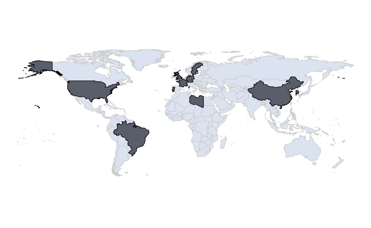
As can be seen on this map, this cluster is relatively representative of all the main country typologies, and represents almost all continents. This is very important in order not to distort the analyses. Indeed, if the observations represented only one typology of State or emanated from only one continent, this would lead to generalize specific results to a given situation. For example, selecting only European countries does not allow us to visualize the dynamics of this pandemic on a global scale.
Thus the selection consists of :
Brazil: located in South America, Brazil is a poor country whose management of the crisis is strongly debated at the international and national level with a resignation of the politicians in charge of the management of the health system. In addition, Brazil has a large number of urban slums, which compromises the effectiveness of lockdown measures. Finally, the country’s health system was in serious trouble even before crisis’s emergence.
China: Located in Asia, China is a reatively rich country is the epicenter of the crisis, the local government of Wuhan tried to hide the emergence of this epidemic and therefore slowed down the establishment of lockdown measures by the central government. China has very good figures which seem to be more related to the strong control of the press by the government than to the real effectiveness of the lockdown measures taken.
France: Located in Western Europe, France is a wealthy country often cited in the past for its very efficient healthcare system. In 2000, France was ranked first in the WHO’s world ranking of health systems, but it has now fallen to 15th place due to the savings made in the health system and its inadequate management. By taking action relatively late, France has avoided the collapse of its health system, but has some of the worst figures in the world. This is partly due to the fairly accurate counting it does compared to other countries.
Germany: Located in Europe, Germany is a rich country and seems to be going through the crisis well as well as being seens as an example by having a low mortality rate as well as a non-total and regionalized lockdown. Germany quickly conducted testing campaigns that enabled it to contain as far as possible the outbreaks of the pandemic on its territory.
Libya: located in Africa, Libya is a country at war which had a relatively functional health system before the health crisis. However the figures for the impact of the pandemic on the country seem to be inaccurate and underestimated due to a lack of testing. For the part of the country currently controlled by the central government, however, measures were taken very early on which probably helped to limit the spread of the virus.
Portugal: Located in Southern Europe, Portugal is a country in economic difficulty following the financial crisis of 2008. This has resulted in massive cost-savings at the expense of the healthcare system, which has suffered heavy staff cuts. However, Portugal, relatively far from the main global communication routes, took advantage of the additional time before the first patient appeared on its territory to take strong and rapid measures. This is now reflected in the excellent figures that the country is reporting. It is an illustration of the success of a good management of the health crisis and proves that the quality of the health system alone is not enough to get through a pandemic with serenity.
The Republic of Korea: Located in Asia, the Republic of Korea is a wealthy country accustomed to the management of epidemics. In 2015, South Korea faced the MERS virus which led it to maintain very high preventive measures and response capacities in case of an epidemic or pandemic. The population is also aware of the cleanliness of public spaces and numerous are those who protect themselves on a daily basis by fear of illness.This has led the country to be the world’s number one example in the management of this crisis, and has allowed the country to avoid lockdown sparing it the economic consequences it induces.
Sweden: Located in Northern Europe, Sweden is a very wealthy country that has made the radical choice not to confine itself in any way. While it does not have more catastrophic figures than France or the United Kingdom, it does have more catastrophic figures compared to its Nordic neighbors such as Norway, Denmark, and Finland. Indeed, by being far removed from the world’s main trade routes, Sweden could have avoided many of the deaths it recorded. This is directly due to the strategy it has put in place which is based on collective immunity, in total opposition to its neighbours.
United Kingdom: Located in Western Europe, the United Kingdom is a wealthy country that took action very late and is now feeling the full effects of the savings that have been made in the healthcare system for many years. The Prime Minister of the United Kingdom initially opted for the Swedish strategy based on collective immunity, before changing strategy and opting for population lockdown. This led to confusion and a lack of preparation in a country that was spared at the beginning of the crisis. Today the United Kingdom has the 4th worst figures among developed countries and the worst of this selection.
United States of America: Located in North America, the United States is a wealthy country with a relatively good healthcare system. The United States has been slow to confine its population and some states have chosen not to confine. The mortality figures from covid-19 classifies the United States as one of the worst countries in the world even though a massive testing campaign is being performed. However, the campaign has been relatively successful in containing the epidemic, despite the total lack of coordination by the federal government, which, like Brazil, is experiencing deep divisions between the specialists in charge of managing the health crisis and the president.
An initial analysis of the number of acute care beds available, among the countries making public their data within the selection of the ten countries, allows to perceive marked disparities in hospital equipment in spite of the relative homogeneity in terms of hospital infrastructure of this cluster.
acute_care_bed <- data.frame(Country = c("France","Germany","Portugal","Sweden",
                                         "Republic of Korea", "United Kingdom", "United States"),
                             Acute_bed = c(309,602,325,204,714,211,244))

ggplot(acute_care_bed) +
 aes(x = Country, y = Acute_bed, fill = Country) +
  geom_col() +
  geom_text(aes(label=Acute_bed), vjust=3.8, color="white", size=4) +
  scale_y_continuous("Acute care beds", limits = c(0,750)) +
  ggthemes::theme_wsj(base_size = (9),color = "white", base_family = "sans", title_family = "mono") +
  ggtitle("Acute care beds in 2017 \nper 100,000 inhabitants")  +
  theme(legend.position = "none",
        axis.text.x = element_text(margin = margin(t = .3, unit = "cm"), angle = 11),
        axis.title=element_text(size=10), axis.title.x = element_blank(),
        axis.title.y = element_text(face = "bold", colour = "#5a5e6b", size = 9))
This chart shows that the number of intensive care beds available per 100,000 population in 2017 varies significantly, from 714 in the Republic of Korea to only 204 in Sweden. Two countries, France and Portugal, appear in the average of this selection with 309 and 325 beds available per 100,000 inhabitants respectively. This variability is interesting because it depicts a very different initial situation depending on the country, and therefore a response strategy that will be impacted by it.
Analysis of mortality rates among the population shows a clear distinction between two groups of countries.
library(ggplot2)
library(ggthemes)

ggplot(dataset_covid_10_countries) +
 aes(x = Country, y = Death.Ratio.Population, fill = Country) +
 geom_col() +
  geom_text(aes(label=round(Death.Ratio.Population)), vjust=-0.4, size=4) +
  scale_y_continuous("Deaths per millions inhabitants", limits = c(0,600)) +
  scale_x_discrete(labels=c("United States of America" = "United States"),
                   limits=c("Brazil", "China", "Germany", "Libya", "Portugal", "Republic of Korea",
                            "France", "Sweden", "United Kingdom", "United States of America")) +
  scale_fill_discrete(name = "Country", labels = c("Brazil", "China", "France", "Germany", "Libya",
                                                   "Portugal", "Republic of Korea", "Sweden",
                                                   "United Kingdom", "United States of America")) +
  ggthemes::theme_wsj(base_size = (9),color = "white", base_family = "sans", title_family = "mono") +
  ggtitle("Covid-19 deaths \namong the population by country") +
  theme(legend.position = "none",
        axis.text.x = element_text(margin = margin(t = .3, unit = "cm"), angle = 11),
        axis.title=element_text(size=10), axis.title.x = element_blank(),
        axis.title.y = element_text(face = "bold", colour = "#5a5e6b", size = 9))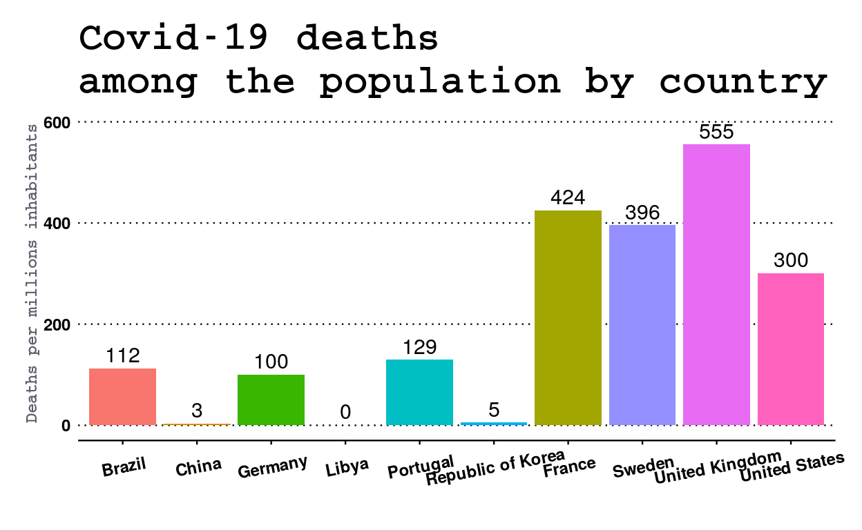
A first group consisting of France, Sweden, the United Kingdom and the United States is easily identifiable. Indeed, the figures obtained by these countries are clearly superior to the others. Thus the United Kingdom records about 550 deaths per million inhabitants, which is more than five times the figure for Germany. As stated in the introduction to this chapter, the Republic of Korea, with the exception of Libya, posted exceptionally low figures, confirming its exemplary handling of the crisis.
If for Germany and the Republic of Korea the figures seem to be right, this is not the case for other countries which are in very different situations such as Brazil which is still at the beginning of the epidemic on its territory or China which, although the cradle of the epidemic, seems to have frozen its figures several months ago.
The following analysis concerns the number of deaths per hundred confirmed cases. This number is directly impacted by the testing policy of countries. Indeed, if the country can practice only relatively few tests, this will induce high mortality rate among those who test positive. Conversely, if the country has the capacity to perform mass testing like this, it improves its rate.
library(ggplot2)
library(ggthemes)

ggplot(dataset_covid_10_countries) +
 aes(x = Country, y = Death.Ratio.Confirmed , fill = Country) +
 geom_col() +
  geom_text(aes(label=round(Death.Ratio.Confirmed)), vjust=1.9, color="White", size=4) +
  scale_y_continuous("Deaths among confirmed cases", limits = c(0,20)) +
  scale_x_discrete(labels=c("United States of America" = "United States"),
                   limits=c("Brazil", "China", "Germany", "Libya", "Portugal", "Republic of Korea",
                            "France", "Sweden", "United Kingdom", "United States of America")) +
  scale_fill_discrete(name = "Country", labels = c("Brazil", "China", "France", "Germany", "Libya",
                                                   "Portugal", "Republic of Korea", "Sweden",
                                                   "United Kingdom", "United States of America")) +
  ggthemes::theme_wsj(base_size = (9),color = "white", base_family = "sans", title_family = "mono") +
  ggtitle("Covid-19 deaths \nper hundred confirmed cases by country") +
  theme(legend.position = "none",
        axis.text.x = element_text(margin = margin(t = .3, unit = "cm"), angle = 11),
        axis.title=element_text(size=10), axis.title.x = element_blank(),
        axis.title.y = element_text(face = "bold", colour = "#5a5e6b", size = 9))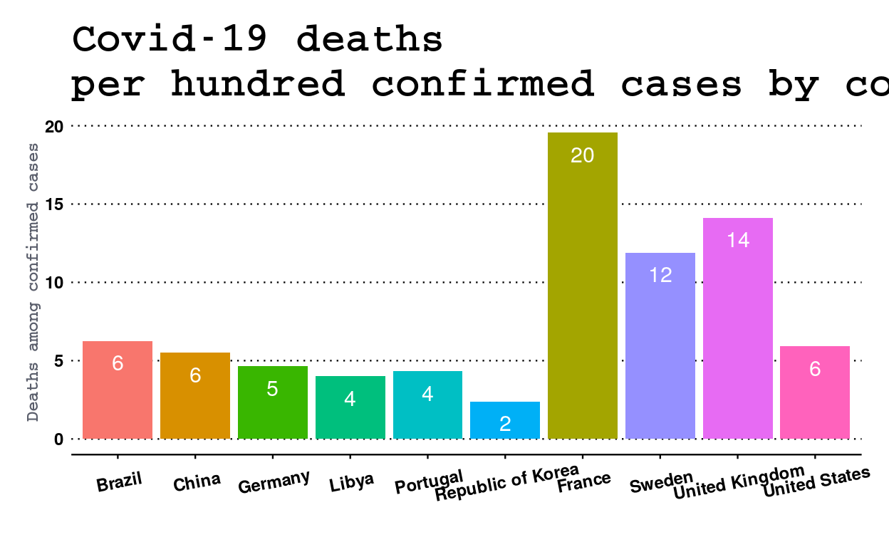
France, which has almost no testing among its population, has a much worse ratio and has the worst selection ratio, with about 20 deaths per hundred tested. In fact, as tests are mainly carried out only on patients admitted to hospital in an already deteriorated health condition, this leads to a higher mortality rate in this ratio. Conversely, the United States, which screens its population on a massive scale, has a very favourable ratio, on a par with China or Brazil and barely higher than that of Germany. However, the United States has the fourth worst ratio in terms of deaths among the population, which shows the caution with which these ratios must be interpreted.
The last but not least graph looks at the time lag between the first confirmed case of covid-19 on the territory of each country and the beginning, or not, of the lockdown measures.
library(dplyr)
library(magrittr)

lockdown <- data.frame(Country = c("Brazil", "China", "France", "Germany", "Libya",
                                   "Portugal", "United Kingdom", "United States"),
                       first_case = c("26.02.20", "17.11.19", "24.01.20", "28.01.20",
                                      "25.03.20", "02.03.20", "31.01.20", "20.01.20"),
                       lockdown_date = c("17.03.20", "23.01.20", "17.03.20", "23.03.20",
                                         "22.03.20", "19.03.20", "23.03.20", "22.03.20"))

lockdown %<>%
  mutate(first_case = as.Date(first_case, format= "%d.%m.%Y"))
lockdown %<>%
  mutate(lockdown_date = as.Date(lockdown_date, format= "%d.%m.%Y"))


lockdown$lockdown_delay <- lockdown$lockdown_date - lockdown$first_case

ggplot(lockdown) +
 aes(x = Country, y = lockdown_delay, fill = Country) +
  geom_col() +
  geom_text(aes(label=round(lockdown_delay)), vjust=-0.15, size=4) +
  scale_y_continuous("delay in days", limits = c(-5,75)) +
  ggthemes::theme_wsj(base_size = (9),color = "white", base_family = "sans", title_family = "mono") +
  ggtitle("Days between first case and country's lockdown")  +
  theme(legend.position = "none",
        axis.text.x = element_text(margin = margin(t = .3, unit = "cm"), angle = 11),
        axis.title=element_text(size=10),
        axis.title.x = element_blank(),
        axis.title.y = element_text(face = "bold", colour = "#5a5e6b", size = 9))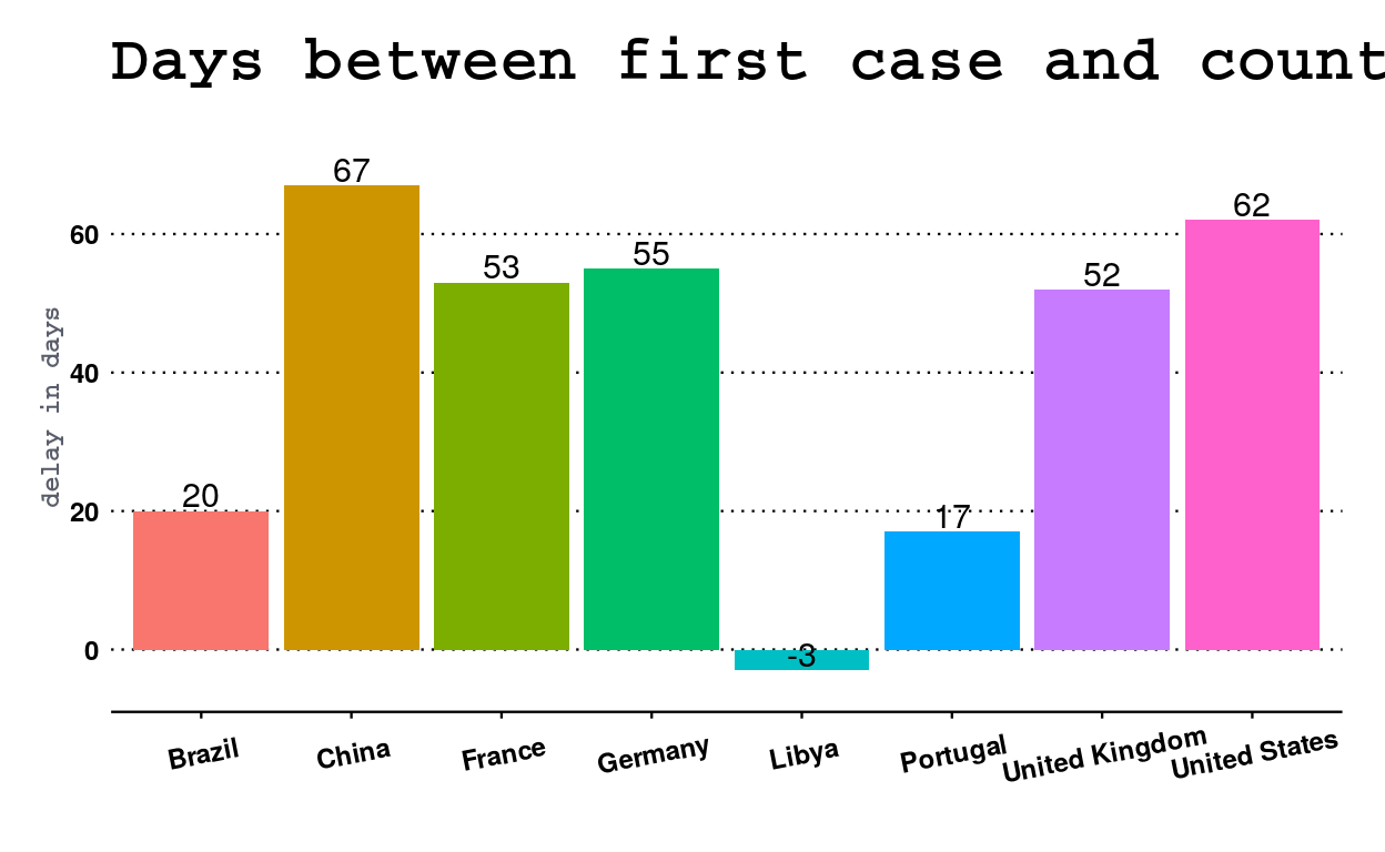
As shown in this graph, some countries, such as Portugal, have reacted very quickly to the presence of the virus on their territories by establishing a generalized containment of the population in only 17 days. Other countries such as China and the United States took very late measures with 67 and 62 days respectively. France is in the average of this selection by confining its population within 53 days, 3 days faster than its neighbour Germany. However, it should not be forgotten that countries such as Portugal and the United Kingdom were hit much later than others, although the United Kingdom did not take advantage of this to prepare for the pandemic.
Finally, some specific cases are to be commented like that of the Republic of Korea and Sweden which chose not to confine their population at all, or Libya which took restrictive measures, more than confinement, 3 days before the first case of covid-19 on its territory.
tl;dr
#Retrieving DEMOCRACY INDEX from Sherbrooke University (EIU.DEMO.GLOBAL, 2017, 163 Countries)

Democracy.Index =c( 2.55, 7.24, 5.98, 3.56, 8.61, 3.62, 1.93, 6.96, 4.11, 9.09, 8.42, 2.65, 2.71, 5.43,
                    3.13, 7.78, 5.61, 5.08, 5.49, 4.87, 7.81, 6.86, 7.03, 4.75, 2.33, 3.63, 3.61, 9.15,
                    7.88, 1.52, 7.84, 3.1, 7.59, 6.67, 3.71, 3.25, 1.61, 1.08, 8, 7.88, 3.93, 6.63, 3.31,
                    9.22, 2.76, 6.66, 3.36, 2.69, 6.02, 2.37, 8.08, 7.79, 3.03, 7.98, 3.42, 9.03, 7.8, 3.61,
                    4.06, 5.93, 6.69, 7.29, 5.86, 3.14, 1.81, 1.98, 6.46, 4.03, 5.72, 6.64, 7.23, 6.39, 4.09,
                    2.45, 9.15, 9.58, 7.79, 7.98, 7.29, 7.88, 3.87, 3.06, 5.11, 5.11, 3.85, 2.37, 6.64, 7.25,
                    4.72, 5.23, 2.32, 7.41, 8.81, 5.57, 5.11, 6.54, 5.49, 5.64, 4.87, 8.22, 3.82, 6.41, 5.94,
                    6.5, 5.69, 4.02, 3.83, 6.31, 5.18, 4.66, 3.76, 4.44, 9.87, 9.26, 3.04, 5.09, 1.95, 4.26,
                    7.08, 6.03, 6.31, 8.89, 6.49, 6.71, 6.67, 7.84, 3.19, 6.44, 8.53, 3.17, 3.19, 6.43, 6.15,
                    6.41, 4.66, 6.32, 7.16, 7.5, 2.15, 6.48, 9.39, 9.03, 6.76, 1.43, 1.93, 7.73, 5.47, 1.5,
                    7.62, 4.63, 7.19, 3.05, 7.04, 6.32, 1.72, 4.88, 5.69, 8.12, 3.87, 3.08, 2.07, 5.68, 3.16)

# Retrieving ISO COUNTRY CODE from Sherbrooke University

ISO = c("AFG", "ZAF", "ALB", "DZA", "DEU", "AGO", "SAU", "ARG", "ARM", "AUS", "AUT", "AZE", "BHR", "BGD", "BLR",
        "BEL", "BEN", "BTN", "BOL", "BIH", "BWA", "BRA", "BGR", "BFA", "BDI", "KHM", "CMR", "CAN", "CPV", "CAF",
        "CHL", "CHN", "CYP", "COL", "COM", "COG", "COD", "PRK", "KOR", "CRI", "CIV", "HRV", "CUB", "DNK", "DJI",
        "DOM", "EGY", "ARE", "ECU", "ERI", "ESP", "EST", "SWZ", "USA", "ETH", "FIN", "FRA", "GAB", "GMB", "GEO",
        "GHA", "GRC", "GTM", "GIN", "GNQ", "GNB", "GUY", "HTI", "HND", "HUN", "IND", "IDN", "IRQ", "IRN", "IRL",
        "ISL", "ISR", "ITA", "JAM", "JPN", "JOR", "KAZ", "KEN", "KGZ", "KWT", "LAO", "LSO", "LVA", "LBN", "LBR",
        "LBY", "LTU", "LUX", "MKD", "MDG", "MYS", "MWI", "MLI", "MAR", "MUS", "MRT", "MEX", "MDA", "MNG", "MON",
        "MOZ", "MMR", "NAM", "NPL", "NIC", "NER", "NGA", "NOR", "NZL", "OMN", "UGA", "UZB", "PAK", "PAN", "PNG",
        "PRY", "NLD", "PER", "PHL", "POL", "PRT", "QAT", "ROM", "GBR", "RUS", "RWA", "SLV", "SEN", "YUG", "SLE",
        "SGP", "SVK", "SVN", "SDN", "LKA", "SWE", "CHE", "SUR", "SYR", "TJK", "TWN", "TZA", "TCD", "CZE", "THA",
        "TMP", "TGO", "TTO", "TUN", "TKM", "TUR", "UKR", "URY", "VEN", "VNM", "YEM", "ZMB", "ZWE")

# Creation of a dataframe called 'democracy'
democracy = data.frame(ISO,Democracy.Index)

# Ordering democracy dataframe by alphabetical order on iso country code
democracy <- democracy[order(ISO),]

#Writing of the democracy index excel file
library(writexl)
write_xlsx(x = democracy, path = "Datasets/dataset_democracy_index.xlsx", col_names = TRUE)

#Retrieving PRESS LIBERTY INDEX from Sherbrooke University (PF.LIB.PRESS.RSF.IN, 2017, 166 Countries)

PRESS.LIBERTY.INDEX =c( 39.46, 20.12, 29.92, 42.83, 14.97, 40.42, 66.02, 25.07, 30.38, 16.02, 13.47, 56.4, 58.88,
                        48.36, 52.43, 12.75, 30.32, 30.73, 33.88, 27.83, 24.93, 33.58, 35.01, 23.85, 55.78, 42.07,
                        41.59, 16.53, 18.02, 36.12, 20.53, 77.66, 19.79, 41.47, 24.33, 36.73, 52.67, 84.98, 27.61,
                        11.93, 30.42, 29.59, 71.75, 10.36, 70.54, 26.76, 55.78, 39.39, 33.64, 84.24, 18.69, 13.55,
                        51.27, 23.88, 50.34, 8.92, 22.24, 34.83, 46.7, 27.76, 17.95, 30.89, 39.33, 33.15, 66.47,
                        30.09, 26.8, 26.36, 43.75, 29.01, 42.94, 39.93, 54.03, 65.12, 14.08, 13.03, 31.01, 26.26,
                        12.73, 29.44, 43.24, 54.01, 31.2, 30.92, 30.45, 33.61, 66.41, 28.78, 18.62, 33.01, 31.12,
                        56.81, 21.37, 14.72, 35.74, 26.71, 46.89, 28.97, 38.27, 42.42, 26.67, 26.49, 48.97, 30.41,
                        28.95, 33.65, 31.05, 41.82, 17.08, 33.02, 31.01, 27.21, 39.69, 7.6, 13.98, 40.46, 35.94, 66.11,
                        43.55, 32.12, 25.07, 35.64, 11.28, 30.98, 41.08, 26.47, 15.77, 39.83, 24.46, 22.26, 49.45, 54.11,
                        27.24, 26.72, 28.05, 30.73, 51.1, 15.51, 21.7, 65.95, 73.56, 48.16, 44.34, 8.27, 12.13, 16.07,
                        81.49, 50.27, 24.37, 30.65, 39.66, 16.91, 44.69, 32.82, 30.75, 20.62, 32.22, 84.19, 52.98, 33.19,
                        17.43, 42.94, 73.96, 65.8, 36.48, 41.44)

#Retrieving ISO COUNTRY CODE from Sherbrooke University

ISO = c("AFG", "ZAF", "ALB", "DZA", "DEU", "AGO", "SAU", "ARG", "ARM", "AUS", "AUT", "AZE", "BHR", "BGD", "BLR", "BEL",
        "BEN", "BTN", "BOL", "BIH", "BWA", "BRA", "BGR", "BFA", "BDI", "KHM", "CMR", "CAN", "CPV", "CAF", "CHL", "CHN",
        "CYP", "COL", "COM", "COG", "COD", "PRK", "KOR", "CRI", "CIV", "HRV", "CUB", "DNK", "DJI", "DOM", "EGY", "ARE",
        "ECU", "ERI", "ESP", "EST", "SWZ", "USA", "ETH", "FIN", "FRA", "GAB", "GMB", "GEO", "GHA", "GRC", "GTM", "GIN",
        "GNQ", "GNB", "GUY", "HTI", "HND", "HUN", "IND", "IDN", "IRQ", "IRN", "IRL", "ISL", "ISR", "ITA", "JAM", "JPN",
        "JOR", "KAZ", "KEN", "KGZ", "KSV", "KWT", "LAO", "LSO", "LVA", "LBN", "LBR", "LBY", "LTU", "LUX", "MKD", "MDG",
        "MYS", "MWI", "MLI", "MAR", "MUS", "MRT", "MEX", "MDA", "MNG", "MON", "MOZ", "MMR", "NAM", "NPL", "NIC", "NER",
        "NGA", "NOR", "NZL", "OMN", "UGA", "UZB", "PAK", "PAN", "PNG", "PRY", "NLD", "PER", "PHL", "POL", "PRT", "QAT",
        "ROM", "GBR", "RUS", "RWA", "SLV", "SEN", "YUG", "SLE", "SGP", "SVK", "SVN", "SOM", "SDN", "SSD", "LKA", "SWE",
        "CHE", "SUR", "SYR", "TJK", "TWN", "TZA", "TCD", "CZE", "THA", "TMP", "TGO", "TTO", "TUN", "TKM", "TUR", "UKR",
        "URY", "VEN", "VNM", "YEM", "ZMB", "ZWE")


#Creation of a DATAFRAME called PRESS
press = data.frame(ISO,PRESS.LIBERTY.INDEX)

#Ordering PRESS DATAFRAME by alphabetical order on ISO COUNTRY CODE
press <- press[order(ISO),]

#TRANSFORMING the REPRESSION PRESS INDEX into a LIBERTY PRESS INDEX
press$Press.Liberty.Index <- 100 - press$PRESS.LIBERTY.INDEX

#DELETING the old REPRESSION COLUMN
press$PRESS.LIBERTY.INDEX <- NULL

#Writing of the PRESS LIBERTY INDEX EXCEL FILE
library(writexl)
write_xlsx(x = press, path = "Datasets/dataset_press_liberty_index.xlsx", col_names = TRUE)

library(readr)

# Downloading data from the Data Europa Portal and saving xlsx file into covid19_cases variable
covid19_cases <- read_csv("https://opendata.ecdc.europa.eu/covid19/casedistribution/csv")

#Deleting unwanted columns
covid19_cases[,1] <- NULL
covid19_cases[,7] <- NULL
covid19_cases[,9] <- NULL

#Renaming columns
names(covid19_cases)[1] <- "Day"
names(covid19_cases)[2] <- "Month"
names(covid19_cases)[3] <- "Year"
names(covid19_cases)[4] <- "Cases"
names(covid19_cases)[5] <- "Deaths"
names(covid19_cases)[6] <- "Country"
names(covid19_cases)[7] <- "ISO"
names(covid19_cases)[8] <- "Population"

head(covid19_cases)

# Writing of the DATASET EXCEL FILE

library(writexl)
write_xlsx(x = covid19_cases, path = "Datasets/dataset_covid19_cases_index.xlsx", col_names = TRUE)

library(WDI)
library(plyr)

#RETRIEVING of the RNB PER INHABITANT for ALL COUNTRIES
RNB_hab_year <- WDI(indicator = "NY.GNP.PCAP.CD",
                   country = "all",
                   start = 2018,
                   end = NULL)


#Handling MISSING VALUES
RNB_hab_year <- na.omit(RNB_hab_year)

#RENAMING of COLUMNS
names(RNB_hab_year)[1] <- "ISO2"
names(RNB_hab_year)[2] <- "Country"
names(RNB_hab_year)[3] <- "RNB.Inhab.Year"


#DELETING UNWANTED COLMUNS
RNB_hab_year$year <- NULL
RNB_hab_year[2] <- NULL

library(readxl)
library(dplyr)

#LOADING WGI dataset VOICE ACCOUNTABILITY
dataset_WGI1 <- read_excel("Datasets/World Governance Indicator/dataset_WGI_2018_Voice_Accountability.xlsx")

#DELETING specific ROWS where values == #N/A

dataset_WGI1 <- subset(dataset_WGI1, Estimate != "#N/A")

#DELETING UNWANTED COLUMNS
dataset_WGI1 <- dataset_WGI1[1:3]

#RENAMING COLUMNS
names(dataset_WGI1)[1] <- "Country"
names(dataset_WGI1)[2] <- "ISO"
names(dataset_WGI1)[3] <- "Voice Accountability"


#################################################################
#LOADING WGI dataset CORRUPTION
dataset_WGI2 <- read_excel("Datasets/World Governance Indicator/dataset_WGI_2018_Corruption.xlsx")

#DELETING specific ROWS where values == #N/A
dataset_WGI2 <- subset(dataset_WGI2, Estimate != "#N/A")

#DELETING UNWANTED COLUMNS
dataset_WGI2 <- dataset_WGI2[1:3]

#RENAMING COLUMNS
names(dataset_WGI2)[1] <- "Country"
names(dataset_WGI2)[2] <- "ISO"
names(dataset_WGI2)[3] <- "Corruption"

#################################################################
#LOADING WGI dataset RULE OF LAW
dataset_WGI3 <- read_excel("Datasets/World Governance Indicator/dataset_WGI_2018_Rule_of_Law.xlsx")

#DELETING specific ROWS where values == #N/A
dataset_WGI3 <- subset(dataset_WGI3, Estimate != "#N/A")

#DELETING UNWANTED COLUMNS
dataset_WGI3 <- dataset_WGI3[1:3]

#RENAMING COLUMNS
names(dataset_WGI3)[1] <- "Country"
names(dataset_WGI3)[2] <- "ISO"
names(dataset_WGI3)[3] <- "Rule of Law"

#################################################################
#LOADING WGI dataset GOVERNMENT EFFECTIVENESS
dataset_WGI4 <- read_excel("Datasets/World Governance Indicator/dataset_WGI_2018_Government_Effectiveness.xlsx")

#DELETING specific ROWS where values == #N/A
dataset_WGI4 <- subset(dataset_WGI4, Estimate != "#N/A")

#DELETING UNWANTED COLUMNS
dataset_WGI4 <- dataset_WGI4[1:3]

#RENAMING COLUMNS
names(dataset_WGI4)[1] <- "Country"
names(dataset_WGI4)[2] <- "ISO"
names(dataset_WGI4)[3] <- "Government Effectiveness"

library(readxl)
library(dplyr)

#IMPORT and SAVING of ISO COUNTRY CODE index
service_capacity_access <- read_excel("Datasets/UHC-service_capacity_access.xlsx")


#MERGING the PRESS LIBERTY INDEX with the DEMOCRACY INDEX (different rows in ISO CODE)
dataset_intermediaire_clustering = merge(press, democracy, by="ISO")

library(readxl)
library(dplyr)

#IMPORT and SAVING of ISO COUNTRY CODE index
ISO_COUNTRY_REDUCED <- read_excel("Datasets/ISO_COUNTRY_TRANSLATION_V2.xlsx")

ISO_COUNTRY_REDUCED <- filter(ISO_COUNTRY_REDUCED, ISO_COUNTRY_REDUCED$ISO != "N/A")

#Writing of the DATASET EXCEL FILE
library(writexl)

write_xlsx(x = ISO_COUNTRY_REDUCED, path = "Datasets/iso_country_reduced.xlsx", col_names = TRUE)

library(dplyr)

#FILTERING DEATHS CASES in the covid19_cases sum up file
sum_deaths_country <- covid19_cases %>%
  group_by(ISO) %>%
  summarize(Deaths.Cases = sum(Deaths, na.rm=TRUE))


#FILTERING CONFIRMED CASES in the covid19_cases sum up file
sum_confirmed_country <- covid19_cases %>%
  group_by(ISO) %>%
  summarize(Confirmed.Cases = sum(Cases, na.rm=TRUE))


#FILTERING POPULATION in the covid19_cases sum up file
 population_country <- covid19_cases %>%
  group_by(ISO) %>%
  summarize(Population = mean(Population, na.rm=TRUE))

library(dplyr)

#LOADINF of the ISO COUNTRY CODE into DATASET INTERMEDIAIRE COVID
dataset_intermediaire_covid <- ISO_COUNTRY_REDUCED

#MERGING DEATH CASES SUM and DATASET INTERMEDIAIRE COVID by ISO code
dataset_intermediaire_covid = merge(sum_deaths_country, dataset_intermediaire_covid, by = "ISO")

#MERGING CONFIRMED CASES SUM and DATASET INTERMEDIAIRE COVID by ISO code
dataset_intermediaire_covid = merge(sum_confirmed_country, dataset_intermediaire_covid, by = "ISO")

#MERGING POPULATION COUNTRY SUM and DATASET INTERMEDIAIRE COVID by ISO code
dataset_intermediaire_covid = merge(population_country, dataset_intermediaire_covid, by = "ISO")


#MOVING COLUMNS in order to have COUNTRY'S NAME as FIRST COLUMN
dataset_intermediaire_covid <- dataset_intermediaire_covid[, c(1, 5, 6, 2, 3, 4)]


dataset_intermediaire_covid$Death.Ratio.Population <- (dataset_intermediaire_covid$Deaths.Cases
                                                       / dataset_intermediaire_covid$Population) * 1000000
dataset_intermediaire_covid$Confirmed.Ratio.Population <- (dataset_intermediaire_covid$Confirmed.Cases
                                                           / dataset_intermediaire_covid$Population) * 1000000
dataset_intermediaire_covid$Death.Ratio.Confirmed <- (dataset_intermediaire_covid$Deaths.Cases
                                                      / dataset_intermediaire_covid$Confirmed.Cases) * 100


dataset_final_covid <- dataset_intermediaire_covid

#Writing of the DATASET EXCEL FILE
library(writexl)

write_xlsx(x = dataset_final_covid, path = "Datasets/dataset_final_covid.xlsx", col_names = TRUE)

library(dplyr)

#INNER_JOIN the RNB PER INHABITANT with the DATASET FINAL (different rows in ISO CODE)
dataset_intermediaire_clustering = inner_join(dataset_intermediaire_covid, RNB_hab_year, by = "ISO2")
dataset_intermediaire_clustering = inner_join(dataset_intermediaire_clustering, press, by = "ISO")
dataset_intermediaire_clustering = inner_join(dataset_intermediaire_clustering, democracy, by = "ISO")

#DELETING UNWANTED COLUMNS
dataset_intermediaire_clustering[3:9] <- NULL


#MERGING VOICE ACCOUNTABILITY and CORRUPTION by ISO code
dataset_WGI2$Country  <- NULL
dataset_intermediaire_WGI = merge(dataset_WGI1, dataset_WGI2, by = "ISO")

#MERGING VOICE ACCOUNTABILITY, CORRUPTION and RULE of LAW by ISO code
dataset_WGI3$Country  <- NULL
dataset_intermediaire_WGI = merge(dataset_intermediaire_WGI, dataset_WGI3, by = "ISO")

#MERGING VOICE ACCOUNTABILITY, CORRUPTION, RULE of LAW and GOVERNMENT EFFECTIVENESS by ISO code
dataset_WGI4$Country  <- NULL
dataset_intermediaire_WGI = merge(dataset_intermediaire_WGI, dataset_WGI4, by = "ISO")

#MERGING VOICE ACCOUNTABILITY, CORRUPTION, RULE of LAW and GOVERNMENT EFFECTIVENESS by ISO code
dataset_intermediaire_WGI$Country  <- NULL
dataset_intermediaire_clustering = merge(dataset_intermediaire_clustering, dataset_intermediaire_WGI, by = "ISO")

library(dplyr)

#TESTING differences existance
dataset_antijoin = anti_join(service_capacity_access, ISO_COUNTRY_REDUCED, by = "Country")

#JOINING SERVICE CAPACITY and ACCESS with ISO COUNTRY file
service_capacity_access_index = full_join(service_capacity_access, ISO_COUNTRY_REDUCED, by = "Country")

service_capacity_access_index <- na.omit(service_capacity_access_index)

names(service_capacity_access_index)[2] <- "Service Capacity and Access"

#SAVING and WRITING of the DATASET EXCEL FILE
library(writexl)

write_xlsx(x = service_capacity_access_index, path = "Datasets/service_capacity_access_index.xlsx", col_names = TRUE)


#MERGING DATASET INTERMEDIAIRE CLUSTERING and SERVICE CAPACITY ACCESS INDEX by ISO code
service_capacity_access_index$Country  <- NULL
dataset_final_clustering = merge(dataset_intermediaire_clustering, service_capacity_access_index, by = "ISO")
dataset_final_clustering$ISO2 <- NULL


#SAVING DATASET FINAL in a EXCEL FILE
write_xlsx(x = dataset_final_clustering, path = "Datasets/dataset_final_WGI_capacity_access.xlsx", col_names = TRUE)

#SAVING DATASET FINAL in a EXCEL FILE
write_xlsx(x = dataset_final_clustering, path = "Datasets/dataset_intermediaire_clustering.xlsx", col_names = TRUE)


library(corrplot)

#LOADIND and SAVING of DATASET FINAL
dataset_intermediaire_covid_correl <- select(dataset_final_covid, 'Population', 'Confirmed.Cases',
                                             'Deaths.Cases', 'Death.Ratio.Population',
                                             'Confirmed.Ratio.Population', 'Death.Ratio.Confirmed')


#COMPUTATION of the CENTERING MATRIX
mcov <- scale(dataset_intermediaire_covid_correl)

mcov <- na.omit(mcov)

#SAVING MCOV as a DATA FRAME
covariance_matrix <- as.data.frame(mcov)


#CORRELATION TEST with HANDLING of MISSING VALUES
mcor <- cor(covariance_matrix, method = "pearson", use = "complete.obs")

#SAVING MCOR as a DATA FRAME
correlation_matrix <- as.data.frame(mcor)

#DISPLAYING of CORRELATION GRAPHIC
col <- colorRampPalette(c("#BB4444", "#EE9988", "#FFFFFF", "#77AADD", "#4477AA"))

corrplot(mcor, method="color", col=col(200), type="upper", order="hclust",
         number.cex = .9, addCoef.col = "black", tl.col="black", tl.srt=45,
         insig = "blank", diag=TRUE )


#COMPUTATION of the P-VALUE COEEFICIENT
library(Hmisc)
p_value <- rcorr(as.matrix(correlation_matrix))

p_value_matrix <- as.data.frame(p_value$P)


#DISPLAYING of SIGNIFICANT P-VALUE CORRELATION GRAPHIC
library(corrplot)

col <- colorRampPalette(c("#BB4444", "#EE9988", "#FFFFFF", "#77AADD", "#4477AA"))

corrplot(p_value$r, method="color", col=col(200), type="upper", order="hclust",
         number.cex = .9, addCoef.col = "black", tl.col="black", tl.srt=45,
         p.mat = p_value$P, sig.level = 0.05, insig = "blank", diag=TRUE )


#LOADIND and SAVING of DATASET FINAL
dataset_intermediaire_clustering_correl <- select(dataset_final_clustering, 'RNB.Inhab.Year', 'Press.Liberty.Index',
                                                  'Democracy.Index', 'Voice Accountability', 'Corruption', 'Rule of Law',
                                                  'Government Effectiveness', 'Service Capacity and Access')

#COMPUTATION of the CENTERING MATRIX
mcov2 <- scale(dataset_intermediaire_clustering_correl)

mcov2 <- na.omit(mcov2)

#SAVING MCOV as a DATA FRAME
covariance_matrix2 <- as.data.frame(mcov2)

#CORRELATION TEST with HANDLING of MISSING VALUES
mcor2 <- cor(covariance_matrix2, method = "pearson", use = "complete.obs")

#SAVING MCOR as a DATA FRAME
correlation_matrix2 <- as.data.frame(mcor2)

#DISPLAYING of CORRELATION GRAPHIC
col <- colorRampPalette(c("#BB4444", "#EE9988", "#FFFFFF", "#77AADD", "#4477AA"))

corrplot(mcor2, method="color", col=col(200), type="full", order="hclust", number.cex = .9,
         addCoef.col = "black", tl.col="black", tl.srt=45, insig = "blank", diag=TRUE )


#COMPUTATION of the P-VALUE COEEFICIENT
library(Hmisc)
p2_value <- rcorr(as.matrix(correlation_matrix2))

p_value_matrix2 <- as.data.frame(p2_value$P)

#DISPLAYING of SIGNIFICANT CORRELATION GRAPHIC
library(corrplot)

col <- colorRampPalette(c("#BB4444", "#EE9988", "#FFFFFF", "#77AADD", "#4477AA"))

corrplot(p2_value$r, method="color", col=col(200), type="full", order="hclust",
         number.cex = .9, addCoef.col = "black", tl.col="black", tl.srt=45,
         p.mat = p2_value$P, sig.level = 0.05, insig = "blank", diag=TRUE )

#TEST SUR LES KMEANS

library(factoextra)
library(purrr)
library(cluster)

#LOADING of the DATASET FINAL2 into DATASET KMEANS1
dataset_kmeans_clustering_temps <- dataset_final_clustering

#Making the FIRST COLUMNS as ROWNAMES
dataset_kmeans_clustering <- dataset_kmeans_clustering_temps[,-1]
rownames(dataset_kmeans_clustering) <- dataset_kmeans_clustering_temps[,1]

#DELETING UNWANTED COLUMNS
dataset_kmeans_clustering <- select(dataset_kmeans_clustering, 'Voice Accountability',
                                    'Rule of Law', 'Service Capacity and Access')

#STANDARDIZATON of the DATASET KMEANS
scale(dataset_kmeans_clustering)

#LOOKING FOR the best number of CLUSTERS by SILHOUETTE method
set.seed(40)

fviz_nbclust(dataset_kmeans_clustering, k.max = 5, kmeans, method = "silhouette")

#CALCULATING the QUALITY of the CLUSTERING depending on NUMBERS of CLUSTERS
gap_stat <- clusGap(dataset_kmeans_clustering, FUN = kmeans,
                    nstart = 25, K.max = 5, B = 50)

#PRINT the RESULT
print(gap_stat, method = "firstmax")

fviz_gap_stat(gap_stat)

#APPLYING the KMEANS ALGORITHM
set.seed(2450)
clusters <- kmeans(dataset_kmeans_clustering, 3, nstart = 25)

fviz_cluster(clusters, data = dataset_kmeans_clustering)

#SAVING the COUNTRY'S CLUSTER NUMBER into DATASET FINAL2
dataset_kmeans_clustering$Cluster <- clusters$cluster


#SAVING DATASET FINAL in a EXCEL FILE
write_xlsx(x = dataset_kmeans_clustering, path = "Datasets/dataset_kmeans_clustering.xlsx", col_names = TRUE)

#Creation of CLUSTER 1 DATAFRAME
#RETRIEVING DATASET KMEANS CLUSTERING to add COUNTRY COLUMN
dataset_cluster_1_temp <- dataset_kmeans_clustering
dataset_cluster_1_temp$Country <- dataset_final_clustering$Country

#FILTERING only COUNTRIES in the CLUSTER 1
dataset_cluster_1 <- filter(dataset_cluster_1_temp, dataset_cluster_1_temp$Cluster == "1")

#MOVING COLUMNS in order to have COUNTRY'S NAME as FIRST COLUMN
dataset_cluster_1 <- dataset_cluster_1[, c(5, 1, 2, 3, 4)]
dataset_cluster_1 <- as.data.frame(dataset_cluster_1)

#SELECTION of COVID NUMBERS for countries in the CLUSTER 1 ONLY
dataset_covid_cluster_1 <- filter(dataset_final_covid, dataset_final_covid$Country %in% dataset_cluster_1$Country)

#COMPUTATION of MEANS for EACH COLUMNS
means_covid_cluster_1 <- colMeans(dataset_covid_cluster_1[4:9])
means_covid_cluster_1 <- as.data.frame(means_covid_cluster_1)

#DELETING ISO2 COLUMN
dataset_covid_cluster_1$ISO2 <- NULL


#RETRIEVING COVID INFORMATIONS by COUNTRY
dataset_covid_10_countries <- subset(dataset_covid_cluster_1, dataset_covid_cluster_1$ISO
                                     %in% c("LBY","BRA","KOR","SWE","FRA","DEU","CHN","USA","GBR","PRT"))

#Creation of CLUSTER 2 DATAFRAME
#RETRIEVING DATASET KMEANS CLUSTERING to add COUNTRY COLUMN
dataset_cluster_1_temp <- dataset_kmeans_clustering
dataset_cluster_1_temp$Country <- dataset_final_clustering$Country

#FILTERING only COUNTRIES in the CLUSTER 2
dataset_cluster_2 <- filter(dataset_cluster_1_temp, dataset_cluster_1_temp$Cluster == "2")

#MOVING COLUMNS in order to have COUNTRY'S NAME as FIRST COLUMN
dataset_cluster_2 <- dataset_cluster_2[, c(5, 1, 2, 3, 4)]
dataset_cluster_2 <- as.data.frame(dataset_cluster_2)

#SELECTION of COVID NUMBERS for countries in the CLUSTER 2 ONLY
dataset_covid_cluster_2 <- filter(dataset_final_covid, dataset_final_covid$Country %in% dataset_cluster_2$Country)

#COMPUTATION of MEANS for EACH COLUMNS
means_covid_cluster_2 <- colMeans(dataset_covid_cluster_2[4:9])
means_covid_cluster_2 <- as.data.frame(means_covid_cluster_2)

#DELETING ISO2 COLUMN
dataset_covid_cluster_2$ISO2 <- NULL

#Creation of CLUSTER 3 DATAFRAME
#RETRIEVING DATASET KMEANS CLUSTERING to add COUNTRY COLUMN
dataset_cluster_1_temp <- dataset_kmeans_clustering
dataset_cluster_1_temp$Country <- dataset_final_clustering$Country

#FILTERING only COUNTRIES in the CLUSTER 3
dataset_cluster_3 <- filter(dataset_cluster_1_temp, dataset_cluster_1_temp$Cluster == "3")

#MOVING COLUMNS in order to have COUNTRY'S NAME as FIRST COLUMN
dataset_cluster_3 <- dataset_cluster_3[, c(5, 1, 2, 3, 4)]
dataset_cluster_3 <- as.data.frame(dataset_cluster_3)

#SELECTION of COVID NUMBERS for countries in the CLUSTER 3 ONLY
dataset_covid_cluster_3 <- filter(dataset_final_covid, dataset_final_covid$Country %in% dataset_cluster_3$Country)

#COMPUTATION of MEANS for EACH COLUMNS
means_covid_cluster_3 <- colMeans(dataset_covid_cluster_3[4:9])
means_covid_cluster_3 <- as.data.frame(means_covid_cluster_3)

#DELETING ISO2 COLUMN
dataset_covid_cluster_3$ISO2 <- NULL

cluster.comparison <- data.frame(Cluster = c("Cluster 1","Cluster 2","Cluster 3"),
                                 Population=c(means_covid_cluster_1[1,],
                                              means_covid_cluster_2[1,],
                                              means_covid_cluster_3[1,]),
                                 Confirmed.Cases = c(means_covid_cluster_1[2,],
                                                     means_covid_cluster_2[2,],
                                                     means_covid_cluster_3[2,]),
                                 Deaths.Cases = c(means_covid_cluster_1[3,],
                                                  means_covid_cluster_2[3,],
                                                  means_covid_cluster_3[3,]),
                                 Death.Ratio.Population = c(means_covid_cluster_1[4,],
                                                            means_covid_cluster_2[4,],
                                                            means_covid_cluster_3[4,]),
                                 Confirmed.Ratio.Population = c(means_covid_cluster_1[5,],
                                                                means_covid_cluster_2[5,],
                                                                means_covid_cluster_3[5,]),
                                 Death.Ratio.Confirmed = c(means_covid_cluster_1[6,],
                                                           means_covid_cluster_2[6,],
                                                           means_covid_cluster_3[6,]))


cluster.comparison <- t(cluster.comparison)

cluster.comparison <- as.data.frame(cluster.comparison)

cluster.comparison <- cluster.comparison[-1,]


library(tidyverse)

colnames(cluster.comparison) = c("Cluster 1", "Cluster 2", "Cluster 3")

rownames(cluster.comparison) <- c("Population", "Confirmed Cases", "Deaths Cases",
                                  "Deaths per millions inhabitants",
                                  "Confirmed cases per millions inhabitants",
                                  "Death ratio per hundred confirmed cases")

library(formattable)
#formattable(cluster.comparison)

formattable(cluster.comparison, align =c("l","c","c","c"),
            list('Cluster 1' = color_tile("#CFCFDC", "#C0C0C0"),
                 'Cluster 2' = color_tile("#CFCFDC", "#C0C0C0"),
                 'Cluster 3' = color_tile("#CFCFDC", "#C0C0C0")))

# Importation de la librairie ggplot2 pour faire la map et dplyr pour manipuler les data
library(ggplot2)


world <- map_data("world")

world <- subset(world, region != "Antarctica")
world <- subset(world, region != "French Southern and Antarctic Lands")

cluster1top10 <- subset(world, region %in% c("Libya", "Brazil", "China", "Germany", "France",
                                             "USA", "South Korea", "Portugal", "UK", "Sweden"))

# Produce a World map
ggplot(data = world, aes(x = long, y = lat, group = group)) +
  geom_polygon(fill = "#dae3ef", color = "#CBCBCC", size = 0.3) +
  geom_polygon(data = cluster1top10, fill = "#5a5e6b", color = "black", size = 0.3) +
  coord_fixed(1) +
  theme_void()

acute_care_bed <- data.frame(Country = c("France","Germany","Portugal","Sweden",
                                         "Republic of Korea", "United Kingdom", "United States"),
                             Acute_bed = c(309,602,325,204,714,211,244))

ggplot(acute_care_bed) +
 aes(x = Country, y = Acute_bed, fill = Country) +
  geom_col() +
  geom_text(aes(label=Acute_bed), vjust=3.8, color="white", size=4) +
  scale_y_continuous("Acute care beds", limits = c(0,750)) +
  ggthemes::theme_wsj(base_size = (9),color = "white", base_family = "sans", title_family = "mono") +
  ggtitle("Acute care beds in 2017 \nper 100,000 inhabitants")  +
  theme(legend.position = "none",
        axis.text.x = element_text(margin = margin(t = .3, unit = "cm"), angle = 11),
        axis.title=element_text(size=10), axis.title.x = element_blank(),
        axis.title.y = element_text(face = "bold", colour = "#5a5e6b", size = 9))

library(ggplot2)
library(ggthemes)

ggplot(dataset_covid_10_countries) +
 aes(x = Country, y = Death.Ratio.Population, fill = Country) +
 geom_col() +
  geom_text(aes(label=round(Death.Ratio.Population)), vjust=-0.4, size=4) +
  scale_y_continuous("Deaths per millions inhabitants", limits = c(0,600)) +
  scale_x_discrete(labels=c("United States of America" = "United States"),
                   limits=c("Brazil", "China", "Germany", "Libya", "Portugal", "Republic of Korea",
                            "France", "Sweden", "United Kingdom", "United States of America")) +
  scale_fill_discrete(name = "Country", labels = c("Brazil", "China", "France", "Germany", "Libya",
                                                   "Portugal", "Republic of Korea", "Sweden",
                                                   "United Kingdom", "United States of America")) +
  ggthemes::theme_wsj(base_size = (9),color = "white", base_family = "sans", title_family = "mono") +
  ggtitle("Covid-19 deaths \namong the population by country") +
  theme(legend.position = "none",
        axis.text.x = element_text(margin = margin(t = .3, unit = "cm"), angle = 11),
        axis.title=element_text(size=10), axis.title.x = element_blank(),
        axis.title.y = element_text(face = "bold", colour = "#5a5e6b", size = 9))

library(ggplot2)
library(ggthemes)

ggplot(dataset_covid_10_countries) +
 aes(x = Country, y = Death.Ratio.Confirmed , fill = Country) +
 geom_col() +
  geom_text(aes(label=round(Death.Ratio.Confirmed)), vjust=1.9, color="White", size=4) +
  scale_y_continuous("Deaths among confirmed cases", limits = c(0,20)) +
  scale_x_discrete(labels=c("United States of America" = "United States"),
                   limits=c("Brazil", "China", "Germany", "Libya", "Portugal", "Republic of Korea",
                            "France", "Sweden", "United Kingdom", "United States of America")) +
  scale_fill_discrete(name = "Country", labels = c("Brazil", "China", "France", "Germany", "Libya",
                                                   "Portugal", "Republic of Korea", "Sweden",
                                                   "United Kingdom", "United States of America")) +
  ggthemes::theme_wsj(base_size = (9),color = "white", base_family = "sans", title_family = "mono") +
  ggtitle("Covid-19 deaths \nper hundred confirmed cases by country") +
  theme(legend.position = "none",
        axis.text.x = element_text(margin = margin(t = .3, unit = "cm"), angle = 11),
        axis.title=element_text(size=10), axis.title.x = element_blank(),
        axis.title.y = element_text(face = "bold", colour = "#5a5e6b", size = 9))

library(dplyr)
library(magrittr)

lockdown <- data.frame(Country = c("Brazil", "China", "France", "Germany", "Libya",
                                   "Portugal", "United Kingdom", "United States"),
                       first_case = c("26.02.20", "17.11.19", "24.01.20", "28.01.20",
                                      "25.03.20", "02.03.20", "31.01.20", "20.01.20"),
                       lockdown_date = c("17.03.20", "23.01.20", "17.03.20", "23.03.20",
                                         "22.03.20", "19.03.20", "23.03.20", "22.03.20"))

lockdown %<>%
  mutate(first_case = as.Date(first_case, format= "%d.%m.%Y"))
lockdown %<>%
  mutate(lockdown_date = as.Date(lockdown_date, format= "%d.%m.%Y"))


lockdown$lockdown_delay <- lockdown$lockdown_date - lockdown$first_case

ggplot(lockdown) +
 aes(x = Country, y = lockdown_delay, fill = Country) +
  geom_col() +
  geom_text(aes(label=round(lockdown_delay)), vjust=-0.15, size=4) +
  scale_y_continuous("delay in days", limits = c(-5,75)) +
  ggthemes::theme_wsj(base_size = (9),color = "white", base_family = "sans", title_family = "mono") +
  ggtitle("Days between first case and country's lockdown")  +
  theme(legend.position = "none",
        axis.text.x = element_text(margin = margin(t = .3, unit = "cm"), angle = 11),
        axis.title=element_text(size=10),
        axis.title.x = element_blank(),
        axis.title.y = element_text(face = "bold", colour = "#5a5e6b", size = 9))
To go further with our pedagogical platform
- Our Coding School
- Our Potential Modules
- Module 1: Data Visualizations
- Module 2: Data Warehouse
- Module 3: News Collection and Analysis
- Module 4: Predictive Modelling
- Module 5: Social Media Collection and Analysis
- Module 6: Mapping
- Module 7: Bibliometrics
- Module 8: Topic Modelling
- Module 9: Covid-19 and International Flows
- Module 10: Covid-19 and Finance
- Module 11: Covid-19 and Public Policies
- Module 12: Covid-19 and Ethics
- Our Databases and APIs