[R Course] Data Visualisation with R: Advanced Static Maps

Learn how to use a shapefile to create a static map with ggplot2.

This course will show you how to create an advanced static map by using a shapefile with ggplot2.

Loading packages

library(maps)
library(ggplot2)
library(dplyr)
library(readr)
library(rgdal)
library(sp)
library(stringr)
library(tidyverse)
library(broom)

Extracting Data

# Data Frame containing info on NYC 2018 murders per borough
NYC2018murders <- read.csv("NYC2018murders.csv", header = TRUE)
head(NYC2018murders)

  borough  weapon record
1   BRONX HANDGUN      1
2   BRONX HANDGUN      1
3   BRONX HANDGUN      1
4   BRONX HANDGUN      1
5   BRONX HANDGUN      1
6   BRONX HANDGUN      1

# NYC boroughs shapefile
# remember, the .zip file must contain at least the .shp, .shx, .dbf, and .prj files 
# components of the shapefile for your shapefile to work properly
Map1 <- readOGR("nycB.shp")

OGR data source with driver: ESRI Shapefile 
Source: "/home/marinel/portfolio/warin/_posts/rcourse-datavisualizationwithr-advancedstaticmaps/nycB.shp", layer: "nycB"
with 5 features
It has 4 fields

# Get "Map1" into tidy format using the tidy() function of the "broom" package.
Map2 <- tidy(Map1)
head(Map2)

# A tibble: 6 x 7
      long     lat order hole  piece group id   
     <dbl>   <dbl> <int> <lgl> <fct> <fct> <chr>
1 1021632. 267934.     1 FALSE 1     0.1   0    
2 1022109. 267751.     2 FALSE 1     0.1   0    
3 1022178. 267762.     3 FALSE 1     0.1   0    
4 1022216. 267734.     4 FALSE 1     0.1   0    
5 1022273. 267697.     5 FALSE 1     0.1   0    
6 1022332. 267664.     6 FALSE 1     0.1   0    

# Add @data back to our Map2 object
Map1$id <- row.names(Map1)

Map2 <- left_join(Map2, Map1@data)
head(Map2)

# A tibble: 6 x 11
    long    lat order hole  piece group id    BoroCode BoroName
   <dbl>  <dbl> <int> <lgl> <fct> <fct> <chr>    <int> <chr>   
1 1.02e6 2.68e5     1 FALSE 1     0.1   0            2 Bronx   
2 1.02e6 2.68e5     2 FALSE 1     0.1   0            2 Bronx   
3 1.02e6 2.68e5     3 FALSE 1     0.1   0            2 Bronx   
4 1.02e6 2.68e5     4 FALSE 1     0.1   0            2 Bronx   
5 1.02e6 2.68e5     5 FALSE 1     0.1   0            2 Bronx   
6 1.02e6 2.68e5     6 FALSE 1     0.1   0            2 Bronx   
# … with 2 more variables: Shape_Leng <dbl>, Shape_Area <dbl>

Data wrangling

# Make sure your data is in the appropriate format
NYC2018murders$borough <- as.character(NYC2018murders$borough)
NYC2018murders$record <- as.character(NYC2018murders$record)
NYC2018murders$weapon <- as.character(NYC2018murders$weapon)
NYC2018murders$record <- as.numeric(NYC2018murders$record)

# Use aggregate function to get the total sum of murders per borough
NYC2018murdersAgg <- aggregate(record~ borough, data = NYC2018murders, sum)  

# Make sure the boroughs are written exactly the same in all the data frames
Map2$BoroName <- str_to_upper(Map2$BoroName)
Map2$BoroName <- as.character(Map2$BoroName)

# rename the column "BoroName" and call it "borough"
names(Map2)[names(Map2) == "BoroName"] <- "borough"

# Join the 2 data frames
FINAL <- left_join(Map2, NYC2018murdersAgg, by = "borough")
head(FINAL)

# A tibble: 6 x 12
    long    lat order hole  piece group id    BoroCode borough
   <dbl>  <dbl> <int> <lgl> <fct> <fct> <chr>    <int> <chr>  
1 1.02e6 2.68e5     1 FALSE 1     0.1   0            2 BRONX  
2 1.02e6 2.68e5     2 FALSE 1     0.1   0            2 BRONX  
3 1.02e6 2.68e5     3 FALSE 1     0.1   0            2 BRONX  
4 1.02e6 2.68e5     4 FALSE 1     0.1   0            2 BRONX  
5 1.02e6 2.68e5     5 FALSE 1     0.1   0            2 BRONX  
6 1.02e6 2.68e5     6 FALSE 1     0.1   0            2 BRONX  
# … with 3 more variables: Shape_Leng <dbl>, Shape_Area <dbl>,
#   record <dbl>

Creating the map

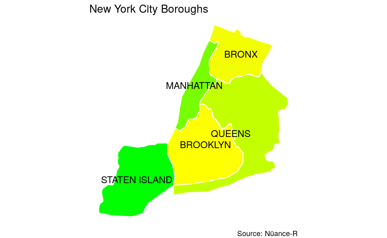
# Create labels
Label <- FINAL %>%
  group_by(borough) %>%
  summarise(label_long = mean(range(long)), label_lat = mean(range(lat)))

# Customize your map
map1 <- ggplot(FINAL, aes(long, lat, group = group))+
        geom_polygon(aes(fill = record), color = "white", show.legend = FALSE)+
        scale_fill_gradient(low = "green", high = "yellow") +
        coord_equal() +
        theme_void() + 
        labs(title = "New York City Boroughs",
        caption = "Source: Nüance-R") +
        geom_text(data = Label, 
            mapping = aes(x = label_long, y = label_lat, label = borough, group = NA),
            cex = 4, col = "black")

# Show the map
print(map1)

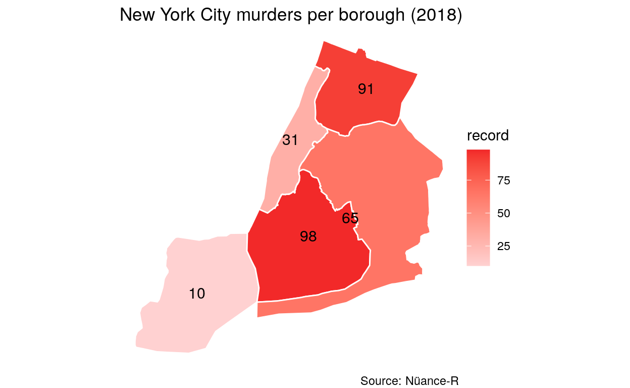
# Create labels
Label <- FINAL %>%
  group_by(borough) %>%
  summarise(label_long = mean(range(long)), label_lat = mean(range(lat)), record = mean(record))

# Customize your map
map <- ggplot(FINAL, aes(long, lat, group = group))+
        geom_polygon(aes(fill = record), color = "white")+
        scale_fill_gradient(low = "#ffd1d1", high = "#f22929") +
        coord_equal() +
        theme_void() + 
        labs(title = "New York City murders per borough (2018)",
        caption = "Source: Nüance-R") +
        geom_text(data = Label, 
            mapping = aes(x = label_long, y = label_lat, label = record, group = NA),
            cex = 4, col = "black")

# Show the map
print(map)