Code chunks
What is a code chunk
- Code chunks in an R Markdown document contain your R code.
- All code chunks start and end with ```.
- A comment in an R chunk is written with a # before the beginning of the sentence.
```{r chunkName}
# This is a comment. Text next to a comment is not processed by R
# Comments will appear on your rendered R markdown document
1+2
```
{r chunkName} contains the language R in this case, and the name of the chunk. Specifying the language is mandatory. Next to the {r}, there is a chunk name. The chunk name is not necessarily required however, it is good practice to give each chunk a unique name to support more advanced knitting approaches
Chunk Options
You can add options to each code chunk. These options allow you to customize how you want your code to be processed or appear on the rendered output (pdf document, html document, etc). Code chunk options are added on the first line of a code chunk after the name, within the curly brackets.
eval
It prevents code from being evaluated. And obviously, if the code is not run, no results will be generated. This is useful for displaying example code, or for disabling a large block of code without commenting each line.
```{r, eval = FALSE}
# your code here
```
eval = FALSE: Do not evaluate (or run) this code chunk when knitting the RMD document. The code in this chunk will still render in our knitted html output, however it will not be evaluated or run by R.
One example of using eval = FALSE is for a code chunk that exports a file such as a figure graphic or a text file. You may want to show or document the code that you used to export that graphic in your html or pdf document, but you don’t need to actually export that file each time you create a revised html or pdf document.
With eval = FALSE you can not see the map.
library(ggplot2)
world <- map_data("world")
world <- subset(world, region != "Antarctica")
world <- subset(world, region != "French Southern and Antarctic Lands")
ggplot(data = world, aes(x = long, y = lat, group = group)) +
  geom_polygon(fill = "#d9b8c9", color = "white", size = 0.5) +
  theme_void() +
  xlab("") +
  ylab("")
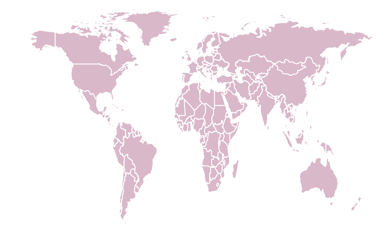
With eval = TRUE you can see the map.
library(ggplot2)
world <- map_data("world")
world <- subset(world, region != "Antarctica")
world <- subset(world, region != "French Southern and Antarctic Lands")
ggplot(data = world, aes(x = long, y = lat, group = group)) +
  geom_polygon(fill = "#d9b8c9", color = "white", size = 0.5) +
  theme_void() +
  xlab("") +
  ylab("")
include
It runs the code, but doesn’t show the code or results in the final document. Use this for setup code that you don’t want cluttering your report.
```{r, include = FALSE}
# your code here
```
Instead of enumerating all kinds of output elements, you can actually hide everything using a single chunk option.
With include = FALSE you cannot see anything at all
With include = TRUE you can see the r chunk and the map
library(ggplot2)
world <- map_data("world")
world <- subset(world, region != "Antarctica")
world <- subset(world, region != "French Southern and Antarctic Lands")
ggplot(data = world, aes(x = long, y = lat, group = group)) +
  geom_polygon(fill = "#d9b8c9", color = "white", size = 0.5) +
  theme_void() +
  xlab("") +
  ylab("")

We use this fonction to hide completely the R chunk and what it does. So the chunk is not visible, but neither is the result. I.e. the code for the map was not shown and so wasn’t the map that came from it. It is usualy used to hide the libraries and all the codes that are not visuals.
echo
It prevents code, but not the results from appearing in the finished file. Use this when writing reports aimed at people who don’t want to see the underlying R code.
echo=FALSE : Hide the code in the output. The code is evaluated when the Rmd file is knit, however only the output is rendered on the output document.
```{r, echo = FALSE}
# your code here
```
With echo = FALSE you cannot see the r chunk, just the map

With echo = TRUE you will see the r chunk and the map
library(ggplot2)
world <- map_data("world")
world <- subset(world, region != "Antarctica")
world <- subset(world, region != "French Southern and Antarctic Lands")
ggplot(data = world, aes(x = long, y = lat, group = group)) +
  geom_polygon(fill = "#d9b8c9", color = "white", size = 0.5) +
  theme_void() +
  xlab("") +
  ylab("")

fig.align
fig.align is as intuitive as it can get. It allows the figure to be placed either on the left, the center or the right.
```{r, fig.align="left"}
# your code here
```plot(cars)

```{r, fig.align="center"}
# your code here
```plot(cars)
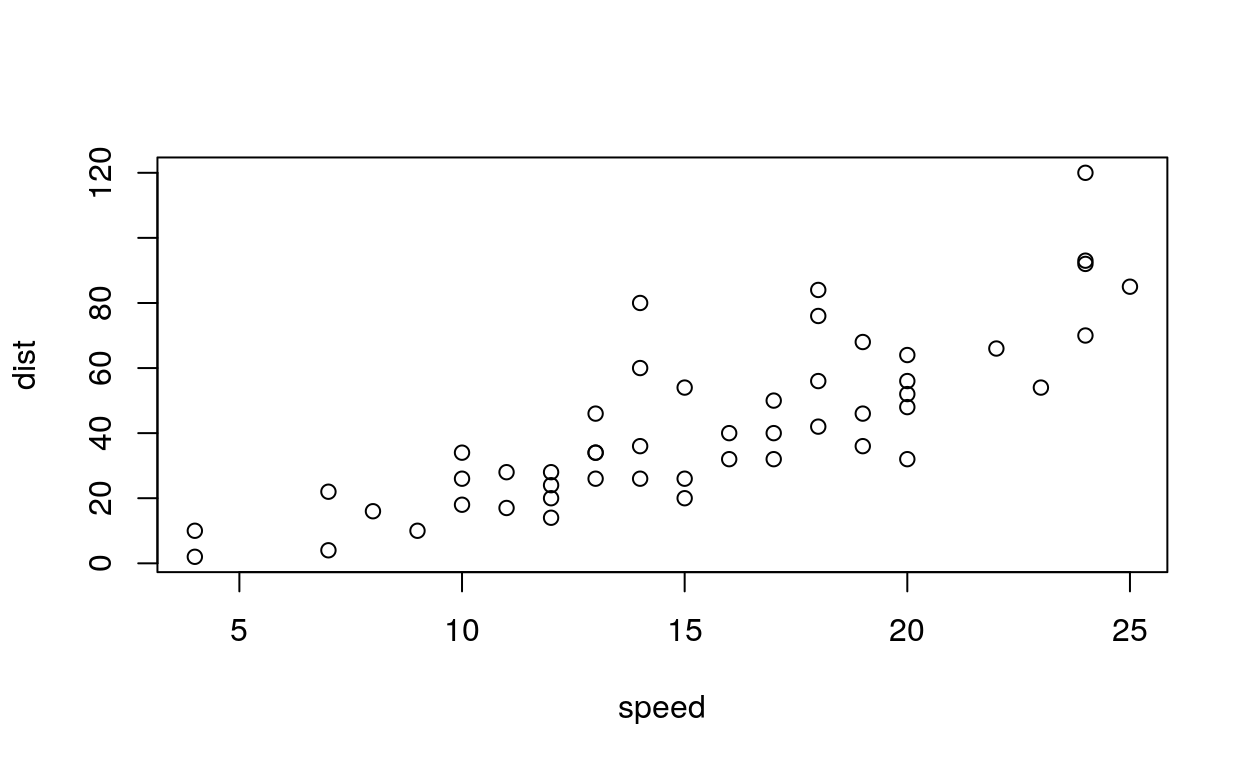
```{r, fig.align="right"}
# your code here
```plot(cars)

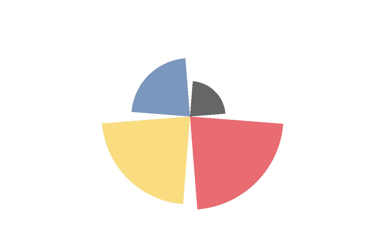
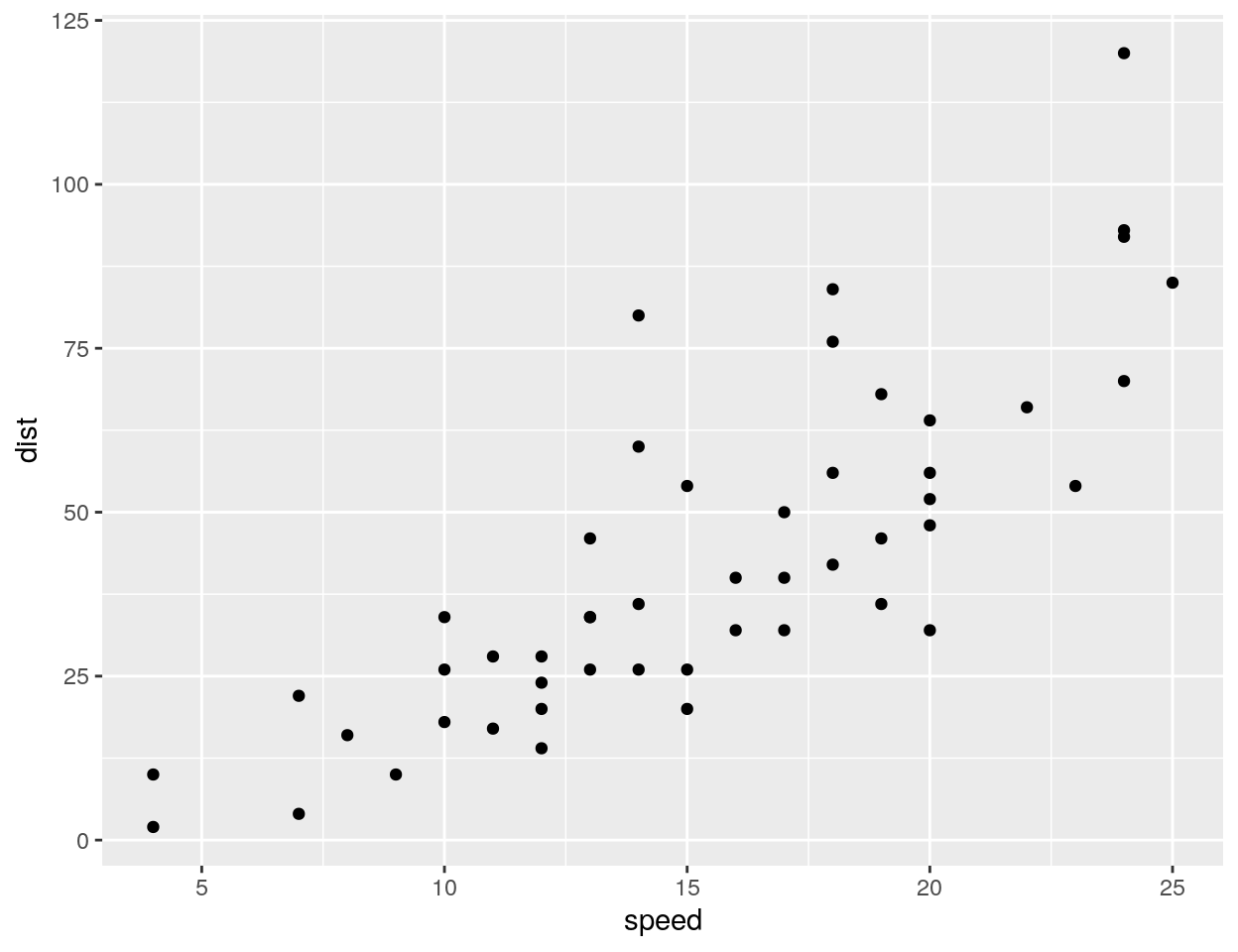
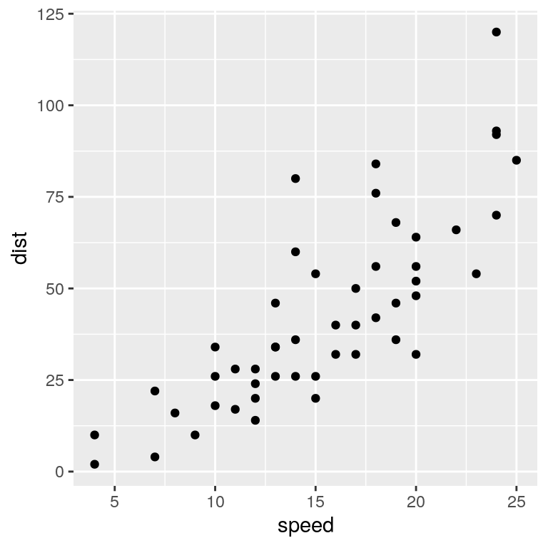
fig.height
The height to use in R for plots created by the chunk (in inches).
```{r, fig.height=5}
# your code here
```
Our graphic with a height of 5
ggplot(cars, aes(speed, dist)) + geom_point()
```{r, fig.height=2}
# your code here
```
Our graphic with a height of 2
ggplot(cars, aes(speed, dist)) + geom_point()
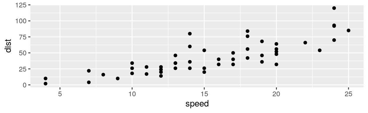
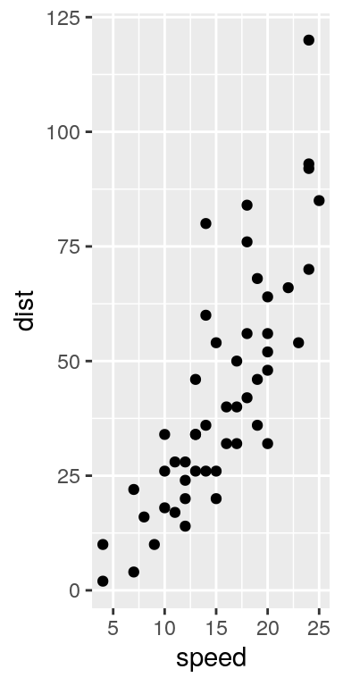
fig.width
The width to use in R for plots created by the chunk (in inches).
```{r, fig.width=4}
# your code here
```
Our graphic with a width of 4
ggplot(cars, aes(speed, dist)) + geom_point()
```{r, fig.width=2}
# your code here
```
Our graphic with a width of 2
ggplot(cars, aes(speed, dist)) + geom_point()
include_graphics
We can use the function include_graphics() from the knitr package which is convenient, as it takes care for the different output formats and provides some more features. Note that online sources are allowed. Don’t forget to load the package knitr previously.
library(knitr)
knitr::include_graphics("image.png")
fig.show
The chunk option fig.show = ‘hide’ allows you to hide printed output.
```{r, fig.show = "hide"}
# your code here
```
results
The chunk option results = hide allows you to evaluate the code but the results or the code will not be rendered on the output document. This is useful if you are viewing the structure of a large object (e.g. outputs of a large data.frame which is the equivalent of a spreadsheet in R).
```{r, results = hide}
# your code here
```
error
error = FALSE causes the render to continue even if code returns an error. This is rarely something you’ll want to include in the final version of your report, but can be very useful if you need to debug exactly what is going on inside your .Rmd. It’s also useful if you’re teaching R and want to deliberately include an error.
The default, error = TRUE causes knitting to fail if there is a single error in the document.
```{r, error = TRUE}
# your code here
```
```{r, error = FALSE}
# your code here
```References
Code Chunks by R for Data Sciencehere
How to Use R Markdown Code Chunks by Leah Wasser here
Yihui’s Blog by Yihui Xie here
R Markdown Reference Guide here
One Little Thing: the knitr Chunk Option include=FALSE here