Introduction
We will use the Netflix dataset, see below.
In linear regression, PCA has been used to achieve two main objectives. The first is used on datasets with an excessive amount of predictor variables. Along with Partial Least Squares Regression, it has been used to reduce dimensionality. There are also methods like ridge regression, Lasso, and remaining regression models with penalties for lowering dimensions (H. Lee, Park, and Lee (2015)). The removal of collinearities between variables is the second purpose of PCR. Because each consecutive main component is orthogonal, PCR was utilised to avoid errors in regression caused by relationships between assumed independent variables (Hadi and Ling, 1998).
EDA
if(!require(devtools)) install.packages("devtools")
devtools::install_github("kassambara/factoextra")
if(!require(FactoMineR)) install.packages("FactoMineR")
if(!require(tidymodels)) install.packages("tidymodels")
if(!require(caret)) install.packages("caret")
Let us remove the Nas:
# A tibble: 6 × 6
    budget popularity   revenue runtime vote_average vote_count
     <dbl>      <dbl>     <dbl>   <dbl>        <dbl>      <dbl>
1 30000000      21.9  373554033      81          7.7       5415
2 65000000      17.0  262797249     104          6.9       2413
3        0      11.7          0     101          6.5         92
4 16000000       3.86  81452156     127          6.1         34
5        0       8.39  76578911     106          5.7        173
6 60000000      17.9  187436818     170          7.7       1886
Creating a train and test dataset:
library(tidymodels)
# Fix the random numbers by setting the seed
# This enables the analysis to be reproducible when random numbers are used
set.seed(222)
# Put 3/4 of the data into the training set
data_split <- initial_split(df, prop = 3/4)

# Create data frames for the two sets:
train_data <- training(data_split)
test_data  <- testing(data_split)
Variable correlation
res <- cor(train_data, method="pearson")
corrplot::corrplot(res, method= "color", order = "hclust", tl.pos = 'n')

Data normalization and standardization
Before performing PCA, all the variables have to be standardised, since PCA is sensitive to data that has not been centered. That is why one of the preprocessing steps in PCA is to normalise data so that it has μ=0 and σ=1. The next step is to perform PCA on matrix X through singular value decomposition. This way we obtain X=UDV′. D is a diagonal matrix consisting of p non-negative singular values, where p is the number of explanatory variables.
\[D = diag[\delta_1, \delta_2, ..., \delta_p] = \begin{bmatrix} \delta_1 & 0 & \cdots & 0 \\ 0 & \delta_2 & \cdots & 0 \\ \vdots & \vdots & \ddots & \vdots \\ 0 & 0 & \cdots & \delta_p \end{bmatrix}\]
This way we obtain p×p matrix V with eigenvectors as columns. Next, using matrix V we calculate matrix Z=XV where each column is one of p principal components. These columns are all orthogonal and ensure no collinearity whatsoever. In order to reduce collinearity we can cut the nuber of components in matrix V to r. This way \(Z_{k \times r} = X_{k \times p}V_{p \times r}\) where \(k\) is the number of observations.
Standardization is a technique in which all the features are centered around zero and have roughly unit variance.
The first line of code below loads the ‘caret’ package, while the second line pre-processes the data. The third line performs the normalization, while the fourth command prints the summary of the standardized variable.
Data normalization is important with PCA to prevent issues created by the different data magnitudes.
library(caret)
# standardization step
train_data.standard <- preProcess(train_data, method = c("center", "scale"))
# normalization step
train_data.norm <- predict(train_data.standard, train_data)
PCA
library("FactoMineR")
res.pca <- PCA(train_data.norm,  graph = FALSE)
library(factoextra)
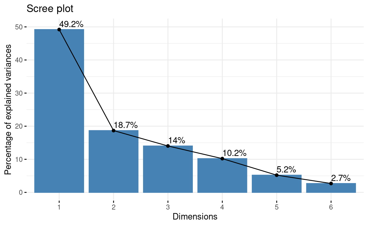
# Extract eigenvalues/variances
get_eig(res.pca)
      eigenvalue variance.percent cumulative.variance.percent
Dim.1  2.9518672        49.197786                    49.19779
Dim.2  1.1206235        18.677058                    67.87484
Dim.3  0.8413958        14.023263                    81.89811
Dim.4  0.6122568        10.204281                    92.10239
Dim.5  0.3125012         5.208353                    97.31074
Dim.6  0.1613556         2.689260                   100.00000
# Visualize eigenvalues/variances
fviz_screeplot(res.pca, addlabels = TRUE, ylim = c(0, 50))
# Extract the results for variables
var <- get_pca_var(res.pca)
var
Principal Component Analysis Results for variables
 ===================================================
  Name       Description
1 "$coord"   "Coordinates for the variables"
2 "$cor"     "Correlations between variables and dimensions"
3 "$cos2"    "Cos2 for the variables"
4 "$contrib" "contributions of the variables"
# Coordinates of variables
head(var$coord)
                 Dim.1       Dim.2       Dim.3        Dim.4
budget       0.8503700 -0.13366457  0.07777397 -0.274505800
popularity   0.7057387  0.05990273 -0.10763660  0.689345278
revenue      0.9118642 -0.15789184  0.01441302 -0.185425694
runtime      0.2211027  0.70847646  0.66961369  0.003070247
vote_average 0.1988716  0.74981378 -0.61162120 -0.153988960
vote_count   0.9004101 -0.10039662 -0.03302425 -0.060014757
                   Dim.5
budget        0.40508418
popularity    0.10571088
revenue      -0.10922307
runtime      -0.02734575
vote_average  0.01942172
vote_count   -0.35238977
# Contribution of variables
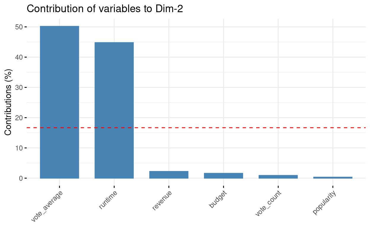
head(var$contrib)
Dim.1 Dim.2 Dim.3 Dim.4 Dim.5
budget 24.497347 1.5943104 0.71889964 12.307487665 52.5096195
popularity 16.872951 0.3202090 1.37695468 77.613982806 3.5759191
revenue 28.168488 2.2246396 0.02468936 5.615729608 3.8174824
runtime 1.656118 44.7910388 53.29032009 0.001539618 0.2392918
vote_average 1.339827 50.1703491 44.45951811 3.872982501 0.1207046
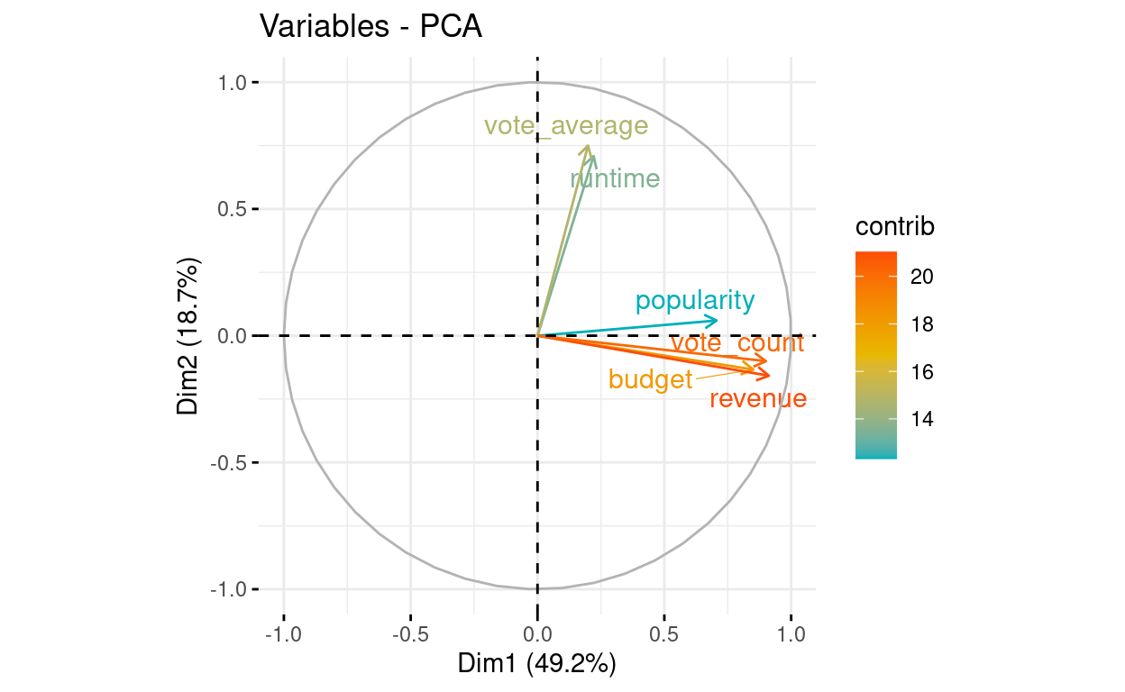
vote_count 27.465270 0.8994531 0.12961813 0.588277804 39.7369826# Control variable colors using their contributions
fviz_pca_var(res.pca, axes = c(1, 2), col.var="contrib",
gradient.cols = c("#00AFBB", "#E7B800", "#FC4E07"),
repel = TRUE # Avoid text overlapping
)
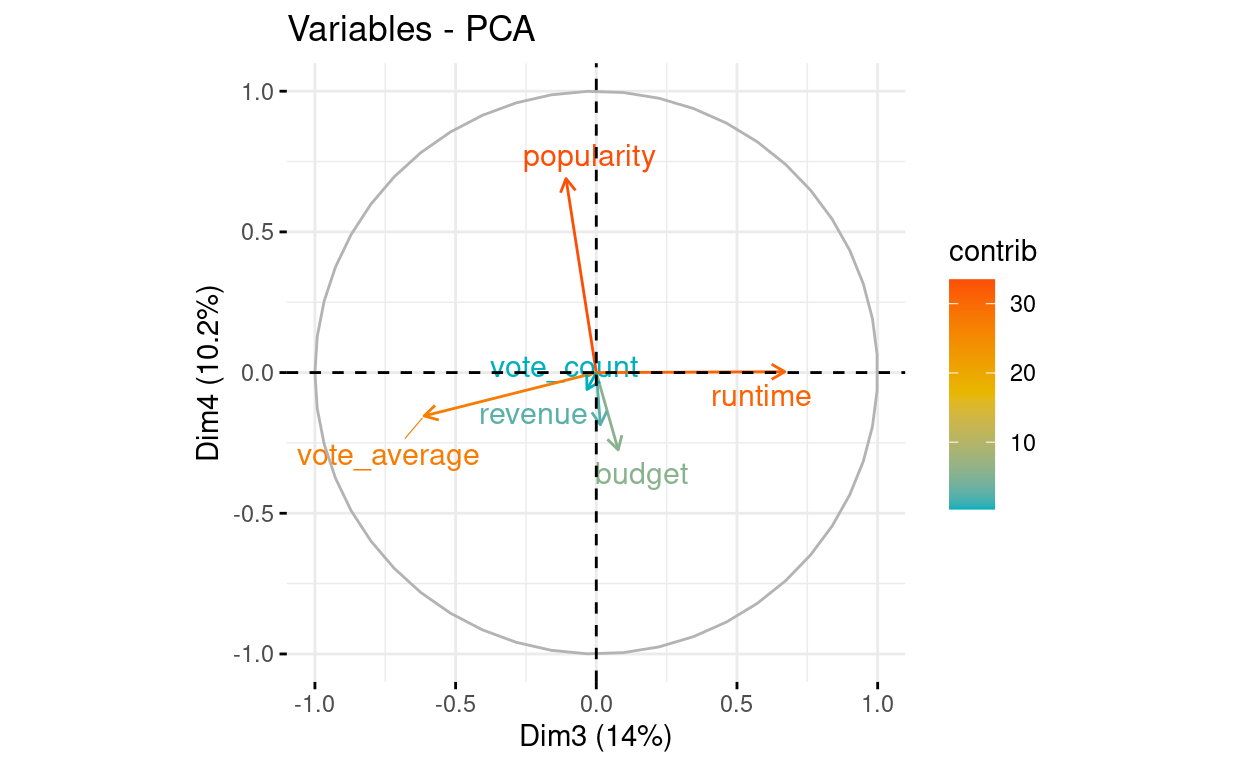
Other dimensions, see the axes argument:
# Control variable colors using their contributions
fviz_pca_var(res.pca, axes = c(3, 4), col.var="contrib",
             gradient.cols = c("#00AFBB", "#E7B800", "#FC4E07"),
             repel = TRUE # Avoid text overlapping
             )
Contributions to dimension 1, see axes = 1:
# Contributions of variables to PC1
fviz_contrib(res.pca, choice = "var", axes = 1, top = 10)
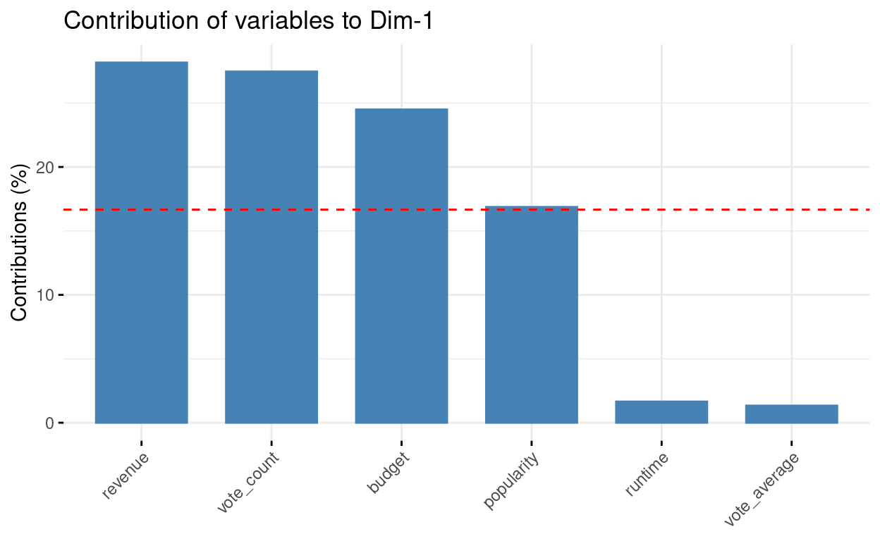
# Contributions of variables to PC2
fviz_contrib(res.pca, choice = "var", axes = 2, top = 10)
# Extract the results for individuals
ind <- get_pca_ind(res.pca)
ind
Principal Component Analysis Results for individuals
 ===================================================
  Name       Description
1 "$coord"   "Coordinates for the individuals"
2 "$cos2"    "Cos2 for the individuals"
3 "$contrib" "contributions of the individuals"
# Coordinates of individuals
head(ind$coord)
Dim.1 Dim.2 Dim.3 Dim.4 Dim.5
1 -0.1412965 -0.48662762 0.5987172 0.7892348 -0.00864576
2 0.8493924 0.37642114 -0.3788261 0.7260344 -0.34173044
3 -0.4888489 -0.07784242 -0.7005577 -0.2279749 -0.01448833
4 -0.4337392 0.51488109 -0.7948625 -0.4212848 -0.04015095
5 0.9457950 1.27375949 0.6160844 -0.2259120 0.31318352
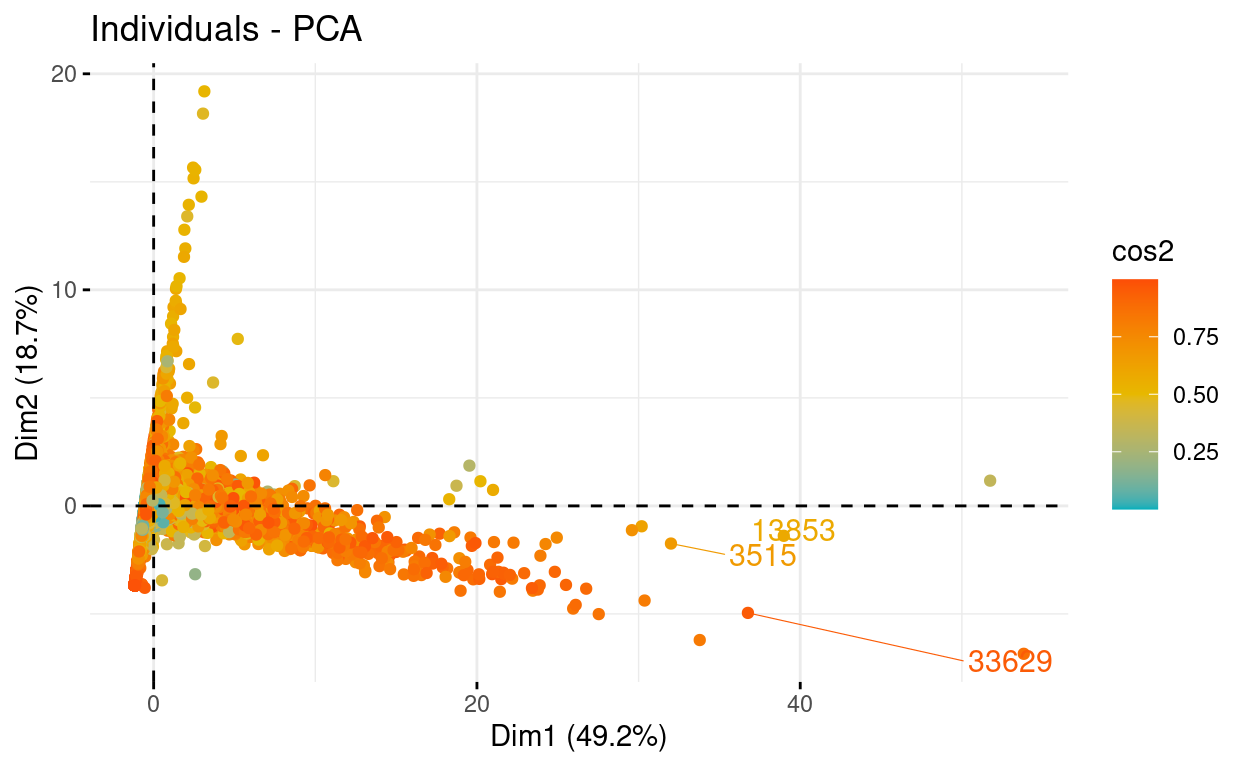
6 0.3812225 0.81715479 -0.8021878 0.3084540 -0.22734262# Graph of individuals
# 1. Use repel = TRUE to avoid overplotting
fviz_pca_ind(res.pca, axes = c(1, 2), col.ind = "cos2",
gradient.cols = c("#00AFBB", "#E7B800", "#FC4E07"),
repel = TRUE # Avoid text overlapping (slow if many points)
)
# Biplot of individuals and variables
fviz_pca_biplot(res.pca, axes = c(1, 2), repel = TRUE)
PCA Regression
Because the PCs \(W_1,..., W_m\) are orthogonal, the problem of multicollinearity is eliminated, and the regression equation will always contain all of the variables in X (because each PC is a linear combination of the variables in X produced by an eigenvector of Z′Z).
Because of the use of orthogonal PCs, PCR is thought to increase the numerical accuracy of regression estimations. (Hadi & Ling, 1998)
Research question: Let us explain popularity by the various dimensions
Now, we need to remove popularity from the variables, and run again the PCA:
train_data.norm.y <- train_data.norm$popularity
train_data.norm$popularity <- NULL
To perform regression, we use the Z matrix consisting of r or p principal components. That way we obtain coefficients from regressing on principal components:
\[\beta_Z = (Z'Z)^{-1}Z'y\]
We can derive the following equation from it:
\[\hat y = Z \beta_Z = (XV) \beta_Z = X(V\beta_Z) = X \beta_X\]
As a result, we can deduce:
\[\beta_X = V \beta_Z\]
res.pca <- PCA(train_data.norm, graph = FALSE)
# Extract the results for individuals
ind <- get_pca_ind(res.pca)
# Coordinates of individuals
head(ind$coord)
       Dim.1       Dim.2      Dim.3       Dim.4       Dim.5
1 -0.3895236 -0.52776067 -0.7022520 -0.15652787  0.02702607
2  0.4839814  0.33417852  0.2926142 -0.50888079  0.53350932
3 -0.3939041 -0.07795885  0.7208728  0.02791553 -0.04646235
4 -0.2912498  0.52497517  0.8446555  0.03768852 -0.06749427
5  0.9148524  1.29927479 -0.5704873  0.35375623 -0.38768880
6  0.1691780  0.78866331  0.7654257 -0.30981914  0.23874354
# We transform the first list within ind into a dataframe to have the dimensions
pcs <- as.data.frame(ind$coord)
Scatterplots
plot(train_data.norm.y, pcs$Dim.1)
plot(train_data.norm.y, pcs$Dim.2)
plot(train_data.norm.y, pcs$Dim.3)
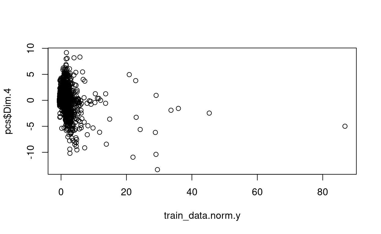
plot(train_data.norm.y, pcs$Dim.4)
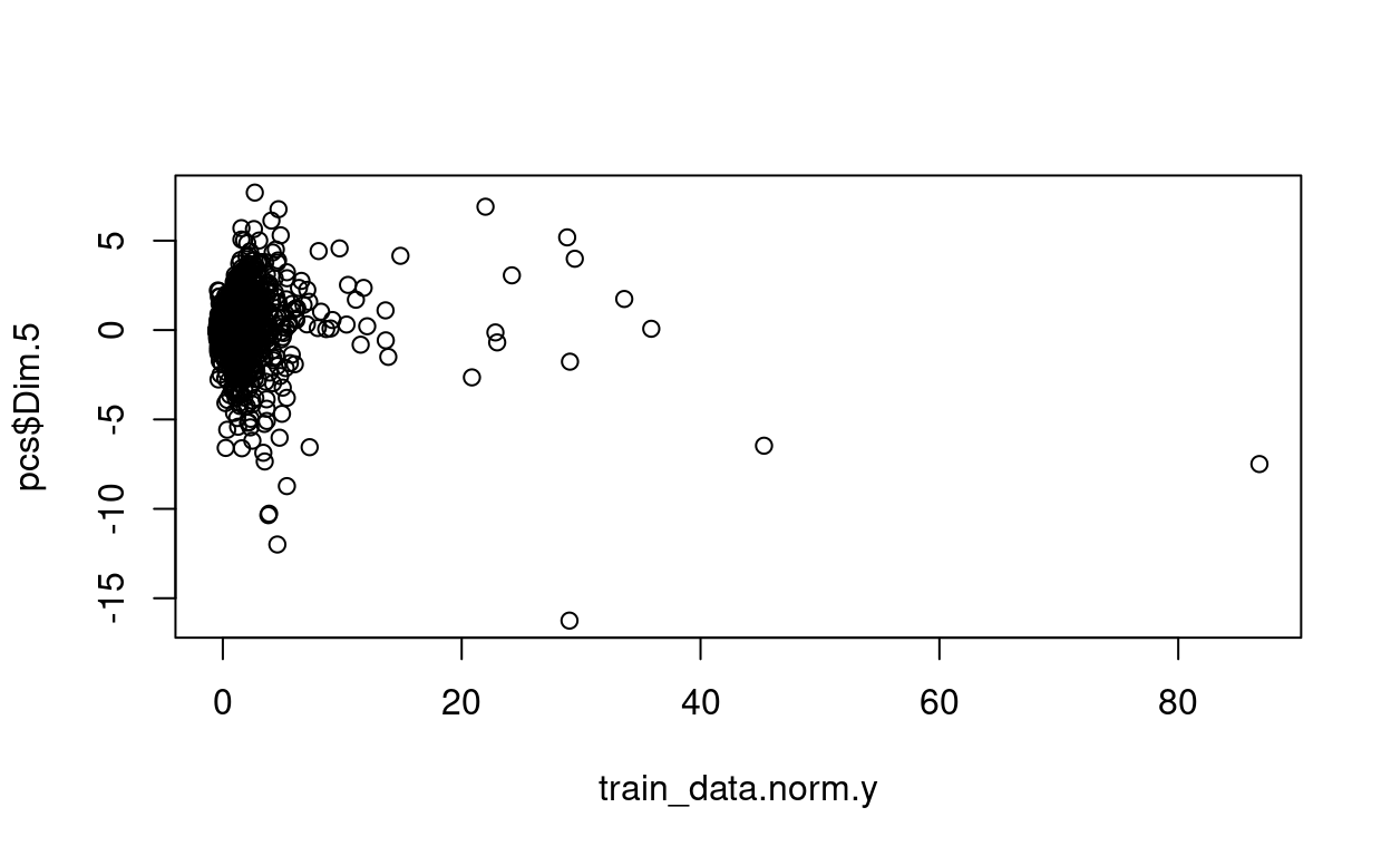
plot(train_data.norm.y, pcs$Dim.5)
Now, let’s combine both the dimensions and the dependent variable:
  train_data.norm.y      Dim.1       Dim.2      Dim.3       Dim.4
1         0.5381243 -0.3895236 -0.52776067 -0.7022520 -0.15652787
2         0.9648818  0.4839814  0.33417852  0.2926142 -0.50888079
3        -0.3247927 -0.3939041 -0.07795885  0.7208728  0.02791553
4        -0.4320840 -0.2912498  0.52497517  0.8446555  0.03768852
5         0.2675722  0.9148524  1.29927479 -0.5704873  0.35375623
6         0.5146545  0.1691780  0.78866331  0.7654257 -0.30981914
        Dim.5
1  0.02702607
2  0.53350932
3 -0.04646235
4 -0.06749427
5 -0.38768880
6  0.23874354
Regression for all the dimensions (does not have to be this way). Remember that we can now which variables contribute to which dimension.
Call:
lm(formula = train_data.norm.y ~ ., data = ols.data)

Residuals:
   Min     1Q Median     3Q    Max
-7.502 -0.273 -0.143  0.104 80.877

Coefficients:
              Estimate Std. Error t value Pr(>|t|)
(Intercept) -2.074e-16  4.475e-03   0.000        1
Dim.1        3.435e-01  2.799e-03 122.733  < 2e-16 ***
Dim.2        3.283e-02  4.231e-03   7.759 8.78e-15 ***
Dim.3        4.051e-02  4.890e-03   8.284  < 2e-16 ***
Dim.4       -2.042e-01  7.845e-03 -26.029  < 2e-16 ***
Dim.5        1.469e-01  1.110e-02  13.236  < 2e-16 ***
---
Signif. codes:  0 '***' 0.001 '**' 0.01 '*' 0.05 '.' 0.1 ' ' 1

Residual standard error: 0.8239 on 33896 degrees of freedom
Multiple R-squared:  0.3213,    Adjusted R-squared:  0.3212
F-statistic:  3209 on 5 and 33896 DF,  p-value: < 2.2e-16
to get the real \(\beta\) coefficients, not from the dimensions/components but from the variables:
beta.Z <- as.matrix(model1$coefficients[2:6]) # [2:6] to capture the 5 dimensions
res.pca2 <- prcomp(train_data.norm)
V <- as.matrix(res.pca2$rotation)
beta.X <- V %*% beta.Z
beta.X
                    [,1]
budget        0.30205877
revenue       0.28493568
runtime       0.09348623
vote_average  0.05085079
vote_count   -0.01553744
Prediction
We have normalized and standardized the train dataset, let us do the same for the test dataset.
library(caret)
# standardization step
test_data.standard <- preProcess(test_data, method = c("center", "scale"))
# normalization step
test_data.norm <- predict(test_data.standard, train_data)
Let us get the dimensions from the test dataset:
res.pca.test <- PCA(test_data.norm, graph = FALSE)
ind.test <- get_pca_ind(res.pca.test)
pcs.test <- as.data.frame(ind.test$coord)
Let us do the prediction:
          1           2           3           4           5
-0.20269180  0.09031361 -0.15442935 -0.08415656  0.48379825
          6
 0.02889301
Remember you can get the variables contributing to these predicted dimension values.
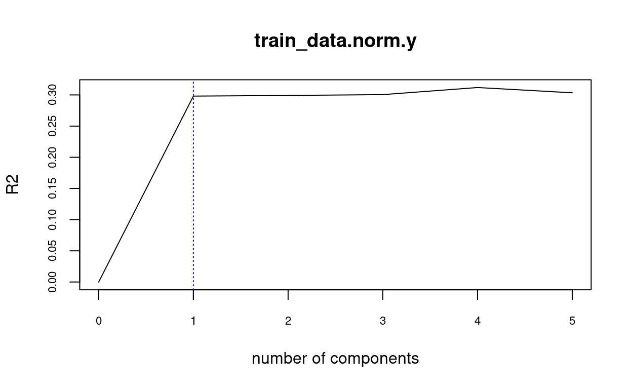
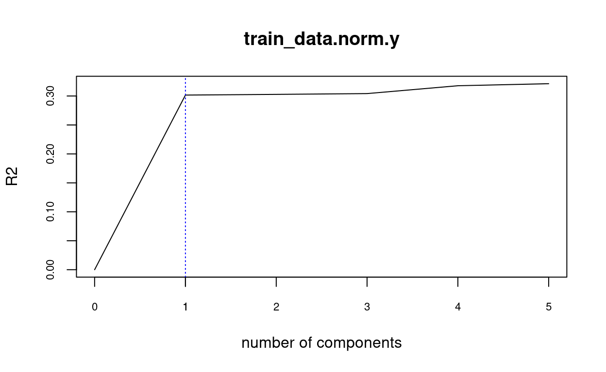
Automatically choosing the number of principal components
When it comes to determining the proper number of primary components, the researchers are divided. Choosing the best principle components as though they were normal variables is one method. Another claim (Hadi and Ling (1998)) is that it is desirable to choose the initial number of PCs that explain the most variance. As a result, some principle components that explain low variance are ruled out. However, this strategy has been criticized because the rejected PCs may actually correlate with the dependent variable (H. Lee, Park, and Lee (2015)).
library(pls)
fit <- pcr(train_data.norm.y ~ ., data = ols.data)
validationplot(fit, val.type="R2", cex.axis=0.7) # change R2 by RMSE or MSE
axis(side = 1, at = c(1), cex.axis=0.7)
abline(v = 1, col = "blue", lty = 3)
With cross validation:
library(pls)
fit2 <- pcr(train_data.norm.y ~ ., data = ols.data, validation = "CV")
validationplot(fit2, val.type="R2", cex.axis=0.7) # change R2 by RMSE or MSE
axis(side = 1, at = c(1), cex.axis=0.7)
abline(v = 1, col = "blue", lty = 3)