This course will teach you how to use the eurostat package.
Loading data
# Load the package
library(eurostat)
library(rvest)

# Get Eurostat data listing
eurostats <- get_eurostat_toc()

# search_eurostat
search_eurostat("waste", type = "table")
# A tibble: 31 x 8
   title code  type  `last update of… `last table str… `data start`
   <chr> <chr> <chr> <chr>            <chr>            <chr>
 1 Gene… ten0… table 22.10.2020       22.10.2020       2004
 2 Gene… ten0… table 22.10.2020       22.10.2020       2004
 3 Wast… ten0… table 22.10.2020       22.10.2020       2004
 4 Gene… sdg_… table 22.10.2020       22.10.2020       2004
 5 Land… t202… table 31.01.2020       27.02.2020       2010
 6 Reco… ten0… table 10.11.2020       10.11.2020       2006
 7 Recy… ten0… table 10.11.2020       10.11.2020       2006
 8 Recy… t202… table 03.07.2020       03.07.2020       1995
 9 Recy… t202… table 26.08.2020       26.08.2020       2008
10 Popu… ten0… table 04.11.2020       04.11.2020       2007
# … with 21 more rows, and 2 more variables: `data end` <chr>,
#   values <chr>
# upload dataframe
dataframe <- get_eurostat("ten00108", type = "label", time_format = "num")
Data Wrangling
# Select only columns you need
data_good<- dplyr::select(dataframe, geo, time, unit, values)

# Delete unwanted rows
data_good <- data_good[-c(1:1704), ]

# Use aggregate function to combine identical data
data_good <- aggregate(values~ geo, data = data_good, sum)

# Remove unwated characters
data_good$geo <- gsub("\\(.*"," ", data_good$geo)
data_good$geo <- gsub("\\-.*"," ", data_good$geo)

# Remove unwated white space
data_good$geo <- trimws(data_good$geo, which = "right", whitespace = "[ \t\r\n]")

# Rename column
names(data_good)[names(data_good) == "geo"] <- "NAME_SORT"

# Delete unwanted rows
datafinal <- data_good[-c(11,12), ]

# Show final data
head(datafinal)
               NAME_SORT    values
1                Austria 188529560
2                Belgium 194761027
3 Bosnia and Herzegovina  12891521
4               Bulgaria 370858822
5                Croatia  16209779
6                 Cyprus   7242410
Visualizing data
# Open your shp file with the readOGR function
Europe <- readOGR("world.shp")
OGR data source with driver: ESRI Shapefile
Source: "/home/marinel/portfolio/warin/_posts/api-eurostat-application/world.shp", layer: "world"
with 241 features
It has 94 fields
Integer64 fields read as strings:  POP_EST NE_ID
# Use "Left join" function to combine your two data frames
Europe@data <- left_join(Europe@data, datafinal, by = "NAME_SORT")
# Create labels
Europe@data$NAME_SORT <- as.character(Europe@data$NAME_SORT)
labels <- sprintf("<strong>%s</strong><br/>%g", Europe@data$NAME_SORT, Europe@data$values) %>% lapply(htmltools::HTML)
# Determinate the intervalls that will be shown in the map legend
bins <- c(0, 100000000, 300000000, 600000000, Inf)
# Choose a color scheme for your map
colors <- colorBin("Reds", domain = Europe@data$values, bins = bins)
# Plot the data using leaflet
leaflet(Europe) %>%
setView(lat = 53.0000, lng = 9.0000, zoom = 3)%>%
addProviderTiles(providers$CartoDB.Positron) %>%
addLegend(pal = colors, values = Europe@data$values, opacity = 0.7, title = NULL, position = "bottomleft") %>%
addPolygons(fillColor = ~colors(Europe@data$values),
weight = 2,
opacity = 1,
color = "white",
dashArray = 1,
fillOpacity = 0.8,
highlight = highlightOptions(weight = 2,
color = "black",
dashArray = 1,
fillOpacity = 0.7,
bringToFront = TRUE),
label = labels
)
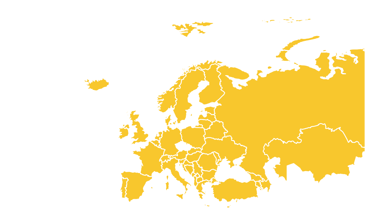
The interactive map above illusrates the total waste in tonne generated by each European Country in 2016. We can easily tell France and Germany are the 2 countries who generated the most waste in 2016.