Basic Usage
You create a Leaflet map with these basic steps:
- Create a map widget by calling leaflet().
- Add layers (i.e., features) to the map by using layer functions (e.g. addTiles, addMarkers, addPolygons) to modify the map widget.
- Repeat step 2 as desired.
- Print the map widget to display it.
Without Marker
With Marker
leaflet() %>%
  addTiles() %>%
  addMarkers(lng=-73.582189, lat=45.517958, popup="The birthplace of Nüance-R")
Widget
The function leaflet() returns a Leaflet map widget, which stores a list of objects that can be modified or updated later. Most functions in this package have an argument map as their first argument, which makes it easy to use the pipe operator %>% in the magrittr package, as you have seen from the example in the Introduction.
Zoom
The map can be zoom in and out. You can play with the leafletOption as follow.
# Set value for the minZoom and maxZoom settings.
leaflet(options = leafletOptions(minZoom = 0, maxZoom = 18)) %>%
  addTiles() %>%
  addMarkers(lng=-73.582189, lat=45.517958, popup="The birthplace of Nüance-R")
Data Object
Both leaflet() and the map layer functions have an optional data parameter that is designed to receive spatial data in one of several forms:
- From base R:
- lng/lat matrix
- data frame with lng/lat columns
- From the sp package: -SpatialPoints[DataFrame]
- Line/Lines
- SpatialLines[DataFrame]
- Polygon/Polygons
- SpatialPolygons[DataFrame]
- From the maps package:
- the data frame from returned from map()
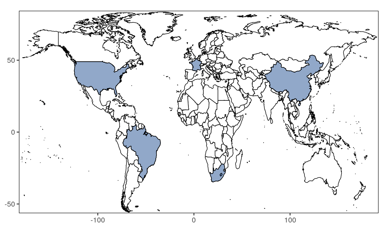
Here an example of the US map with colored states:
leaflet(data = usa_states) %>%
  addTiles() %>%
  addPolygons(fillColor = topo.colors(10, alpha = NULL), stroke = FALSE)
Markers
Data sources
Point data for markers can come from a variety of sources:
- SpatialPoints or SpatialPointsDataFrame objects (from the sp package)
- POINT, sfc_POINT, and sf objects (from the sf package); only X and Y dimensions will be considered
- Two-column numeric matrices (first column is lngitude, second is latitude)
- Data frame with latitude and logitude columns. You can explicitly tell the marker function which columns contain the coordinate data (e.g. addMarkers(lng = ~lngitude, lat = ~Latitude)), or let the function look for columns named lat/latitude and lon/lng/lng/lngitude (case insensitive).
- Simply provide numeric vectors as lng and lat arguments Note that MULTIPOINT objects from sf are not supported at this time.
Icon Markers
Icon markers are added using the addMarkers or the addAwesomeMarkers functions. Their default appearance is a dropped pin. As with most layer functions, the popup argument can be used to add a message to be displayed on click, and the label option can be used to display a text label either on hover or statically.
Leaflet allow you to add multiple markers on a map. As example, let’s create a data frame containing longitude and latitude of a school. You have to search the longitude and latitude for each wanted location.
# Create a data frame with longitude and latitude of campuses.
campuses <- data.frame(country=c("United States", "Brazil", "South Africa", "China", "France", "France", "France"),
                             city=c("Raleigh", "Belo Horizonte", "Cap Town", "Suzhou", "Paris", "Lille", "Sophia Antipolis"),
                             lng=c(-80.793457, -43.940933, 18.423300, 120.599998, 2.349014, 3.05858, 7.25),
                             lat=c(35.782169, -19.912998, -33.918861, 31.299999, 48.864716, 50.63297, 43.7))

campuses
        country             city        lng       lat
1 United States          Raleigh -80.793457  35.78217
2        Brazil   Belo Horizonte -43.940933 -19.91300
3  South Africa         Cap Town  18.423300 -33.91886
4         China           Suzhou 120.599998  31.30000
5        France            Paris   2.349014  48.86472
6        France            Lille   3.058580  50.63297
7 France Sophia Antipolis 7.250000 43.70000leaflet(data = campuses) %>%
addTiles() %>%
addMarkers(lng=~lng, lat=~lat, popup=~country)
Customizing Marker Icons
You can provide custom markers in one of several ways, depending on the scenario. For each of these ways, the icon can be provided as either a URL or as a file path.
One color
For the simple case of applying a single icon to a set of markers, use makeIcon().
greenLeafIcon <- makeIcon(
  iconUrl = "http://leafletjs.com/examples/custom-icons/leaf-green.png",
  iconWidth = 38, iconHeight = 95,
  iconAnchorX = 22, iconAnchorY = 94,
  shadowUrl = "http://leafletjs.com/examples/custom-icons/leaf-shadow.png",
  shadowWidth = 50, shadowHeight = 64,
  shadowAnchorX = 4, shadowAnchorY = 62
)
leaflet(data = campuses) %>%
  addTiles() %>%
  addMarkers(lng=~lng, lat=~lat, popup=~country, icon = greenLeafIcon)
Two colors
Let’s say that you want a different color for one (or more) location. For example, we want the french campus with a red leaf icon.
leafIcons <- icons(
  iconUrl = ifelse(campuses$language == "French",
    "http://leafletjs.com/examples/custom-icons/leaf-red.png",
    "http://leafletjs.com/examples/custom-icons/leaf-green.png"
  ),
  iconWidth = 38, iconHeight = 95,
  iconAnchorX = 22, iconAnchorY = 94,
  shadowUrl = "http://leafletjs.com/examples/custom-icons/leaf-shadow.png",
  shadowWidth = 50, shadowHeight = 64,
  shadowAnchorX = 4, shadowAnchorY = 62
)

leaflet(data = campuses) %>% addTiles() %>%
  addMarkers(~lng, ~lat, icon = leafIcons)
Multiple colors
# Create a column with the continents names for labeling in the map
campuses$continent <- ifelse(campuses$country == c("United States", "Brazil"), "Americas", ifelse(campuses$country == "France", "Europe", "RoW"))


# Create a column containing a code (1, 2, 3 etc.) to match c
campuses$code <- ifelse(campuses$country == c("United States", "Brazil"), 1,
                                ifelse(campuses$country == "France", 2, 3))
getColor <- function(campuses) {
  sapply(campuses$code, function(code) {
  if(code == 1) {
    "green"
  } else if(code == 2) {
    "red"
  } else {
    "orange"
  } })
}

icons <- awesomeIcons(
  icon = 'ios-close',
  iconColor = 'black',
  library = 'ion',
  markerColor = getColor(campuses)
)

leaflet(campuses) %>% addTiles() %>%
  addAwesomeMarkers(~lng, ~lat, icon=icons, label=~as.character(continent))
Marker Clusters
When there are a large number of markers on a map, you can cluster them using the Leaflet.markercluster plug-in. To enable this plug-in, you can provide a list of options to the argument clusterOptions, e.g.
The School has 3 campuses in France. Let’s add them on the map in a cluster.
leaflet(campuses) %>%
  addTiles() %>%
  addMarkers(clusterOptions = markerClusterOptions())
When you zoom in, you can see the markers separately.
Circle Markers
Circle markers are much like regular circles, except that their radius in onscreen pixels stays constant regardless of zoom level.
You can use their default appearance:
leaflet(campuses) %>%
  addTiles() %>%
  addCircleMarkers()
Or customize their color, radius, stroke, opacity, etc.
# Create a palette that maps factor levels to colors
pal <- colorFactor(c("navy", "red"), domain = c("English", "French"))

leaflet(campuses) %>%
  addTiles() %>%
  addCircleMarkers(
    radius = ~ifelse(language == "French", 6, 10),
    color = ~pal(language),
    stroke = FALSE,
    fillOpacity = 0.5
  )
Popups
Popups are small boxes containing arbitrary HTML, that point to a specific point on the map.
You’ve already seen this example above:
leaflet(data = campuses) %>%
  addTiles() %>%
  addMarkers(lng=~lng, lat=~lat, popup=~city)
Another way to have a popup is by using the addPopups() function to add standalone popup to the map.
content <- paste(sep = "<br/>",
  "<b><a href='https://lab.nuance-r.com/'>Nüance-R</a></b>",
  "4200 Saint Laurent Blvd",
  "Montréal, QC H2W2R2"
)

leaflet() %>% addTiles() %>%
  addPopups(lng = -73.582189, lat = 45.517958, content,
    options = popupOptions(closeButton = FALSE)
  )
Labels
A label is a textual or HTML content that can attached to markers and shapes to be always displayed or displayed on mouse over. Unlike popups you don’t need to click a marker/polygon for the label to be shown.
library(htmltools)

leaflet(campuses) %>%
  addTiles() %>%
  addMarkers(~lng, ~lat, label = ~htmlEscape(country))
Customizing Marker Labels
You can customize marker labels using the labelOptions argument of the addMarkers function. The labelOptions argument can be populated using the labelOptions() function. If noHide is false (the default) then the label is displayed only when you hover the mouse over the marker; if noHide is set to true then the label is always displayed.
# Change Text Size and text Only and also a custom CSS
leaflet() %>%
  addTiles() %>%
  setView(-2.349014, 48.864716, 2) %>%
  addMarkers(
    lng = -80.793457, lat = 35.782169,
    label = "Default Label",
    labelOptions = labelOptions(noHide = T)) %>%
  addMarkers(
    lng = -43.940933, lat = -19.912998,
    label = "Label without surrounding box",
    labelOptions = labelOptions(noHide = T, textOnly = TRUE)) %>%
  addMarkers(
    lng = 18.423300, lat = -33.918861,
    label = "label with textsize 15px",
    labelOptions = labelOptions(noHide = T, textsize = "15px")) %>%
  addMarkers(
    lng = 120.599998, lat = 31.299999,
    label = "hidden label with textsize 12px",
    labelOptions = labelOptions(noHide = F, textsize = "10px")) %>%
  addMarkers(
    lng = 2.349014, lat = 48.864716,
    label = "Label w/ custom CSS style",
    labelOptions = labelOptions(noHide = T, direction = "bottom",
      style = list(
        "color" = "red",
        "font-family" = "serif",
        "font-style" = "italic",
        "box-shadow" = "3px 3px rgba(0,0,0,0.25)",
        "font-size" = "12px",
        "border-color" = "rgba(0,0,0,0.5)"
      )))
Labels without markers
You can create labels without the accompanying markers using the addLabelOnlyMarkers function.
leaflet() %>%
  addTiles() %>%
  addLabelOnlyMarkers(data = campuses, lng = ~lng, lat = ~lat, label = ~as.character(city),
                      labelOptions = labelOptions(noHide = T, direction = 'top', textOnly = T))
Shapes
Circles
Circles are added using addCircles(). Circles are similar to circle markers; the only difference is that circles have their radii specified in meters, while circle markers are specified in pixels. As a result, circles are scaled with the map as the user zooms in and out, while circle markers remain a constant size on the screen regardless of zoom level.
When plotting circles, only the circle centers (and radii) are required, so the set of valid data sources is different than for polygons and the same as for markers. See the introduction to Markers for specifics.
leaflet(campuses) %>%
  addTiles() %>%
  addCircles(lng = ~lng, lat = ~lat, weight = 10, radius = ~students * 200, popup = ~city)
Rectangles
Rectangles are added using the addRectangles() function. It takes lng1, lng2, lat1, and lat2 vector arguments that define the corners of the rectangles. These arguments are always required; the rectangle geometry cannot be inferred from the data object.
leaflet() %>%
  addTiles() %>%
  addRectangles(
    lng1=-73.582189, lat1=45.517958,
    lng2=-73.582700, lat2=45.517500,
    fillColor = "transparent"
  )
Tiles
Leaflet supports basemaps using map tiles.
Default OpenStreetMap Tiles
The easiest way to add tiles is by calling addTiles() with no arguments; by default, OpenStreetMap tiles are used.
Third-Party Tiles
Alternatively, many popular free third-party basemaps can be added using the addProviderTiles() function, which is implemented using the leaflet-providers plugin.
As a convenience, leaflet also provides a named list of all the third-party tile providers that are supported by the plugin. This enables you to use auto-completion feature of your favorite R IDE (like RStudio) and not have to remember or look up supported tile providers; just type providers$ and choose from one of the options. You can also use names(providers) to view all of the options.
leaflet() %>% setView(lng = -73.656830 , lat = 45.516136, zoom = 12) %>%
  addProviderTiles(providers$Stamen.Toner)
leaflet() %>% setView(lng = -73.656830 , lat = 45.516136, zoom = 12) %>%
  addProviderTiles(providers$CartoDB.Positron)
leaflet() %>% setView(lng = -73.656830 , lat = 45.516136, zoom = 12) %>%
  addProviderTiles(providers$Esri.NatGeoWorldMap)
Providers Tiles
Leaflet provides a lot of different Tiles. You can found them here.
To use one of these tiles it’s simple. Add providers$ with the name of the desired tile in the funtion addProviderTiles().
Here some example:
OpenTopoMap
leaflet() %>% setView(lng = -73.656830 , lat = 45.516136, zoom = 9) %>%
  addProviderTiles(providers$OpenTopoMap)
Stamen.Watercolor
leaflet() %>% setView(lng = -73.656830 , lat = 45.516136, zoom = 11) %>%
  addProviderTiles(providers$Stamen.Watercolor)
NASAGIBS.ViirsEarthAtNight2012
leaflet() %>% setView(lng = -73.656830 , lat = 45.516136, zoom = 2.5) %>%
  addProviderTiles(providers$NASAGIBS.ViirsEarthAtNight2012)
Esri.WorldTerrain
leaflet() %>% setView(lng = -73.656830 , lat = 45.516136, zoom = 3) %>%
  addProviderTiles(providers$Esri.WorldTerrain)
Combining Tile Layers
You aren’t restricted to using a single basemap on a map; you can stack them by adding multiple tile layers. This generally only makes sense if the front tiles consist of semi transparent tiles, or have an adjusted opacity via the options argument.
leaflet() %>% setView(lng = -73.656830 , lat = 45.516136, zoom = 12) %>%
  addProviderTiles(providers$MtbMap) %>%
  addProviderTiles(providers$Stamen.TonerLines, options = providerTileOptions(opacity = 0.35)) %>%
  addProviderTiles(providers$Stamen.TonerLabels)
Custom Tile URL Template
If you happen to have a custom map tile URL template to use, you can provide it as an argument to addTiles().
You can use addWMSTiles() to add WMS (Web Map Service) tiles. The map below shows the Base Reflectivity (a measure of the intensity of precipitation occurring) using the WMS from the Iowa Environmental Mesonet:
leaflet() %>% addTiles() %>% setView(-93.65, 42.0285, zoom = 4) %>%
  addWMSTiles(
    "http://mesonet.agron.iastate.edu/cgi-bin/wms/nexrad/n0r.cgi",
    layers = "nexrad-n0r-900913",
    options = WMSTileOptions(format = "image/png", transparent = TRUE),
    attribution = "Weather data © 2012 IEM Nexrad"
  )