Chapter 7 Data Wrangling 2/4
7.1 Introduction
What makes R a compiling programming language is its facility to wrangle data on the fly. In this chapter, you will learn the basics of data manipulation. Based on the knowledge acquired in the previous chapters, you will transform datasets in order to prepare them for the chapter 10 which is all about data visualization!
We will use the United Nations Industrial Development Organization (UNIDO) dataset to illustrate this session.
At the end of the chapter, you should be able to:
- add a column to an existing dataframe;
- subset your dataframe based on a variable;
- sort your dataframe;
You will go from a database of 655’350 points to a graphic made of 6 observations.
7.2 Adding & Deleting Variables
Now that you can work with your dataset, you may need to add another column to it. To do so, enter the name of your new column after the $ symbol and assign a value to it.
# Loading the gsheet package
library(gsheet)
# Read data from the URL
dataUnido <- gsheet::gsheet2tbl("https://docs.google.com/spreadsheets/d/1uLaXke-KPN28-ESPPoihk8TiXVWp5xuNGHW7w7yqLCc/edit#gid=416085055")
dataUnido
## # A tibble: 65,536 x 10
## tableCode countryCode year isicCode isicCodeCombina… value tableDefinition…
## <dbl> <dbl> <dbl> <dbl> <chr> <dbl> <dbl>
## 1 1 31 2005 106 106 89 2
## 2 1 31 2006 106 106 82 2
## 3 1 31 2007 106 106 76 2
## 4 1 31 2008 106 106 69 2
## 5 1 31 2009 106 106 55 2
## 6 1 31 2010 106 106 55 2
## 7 1 31 2011 106 106 51 2
## 8 1 31 2012 106 106 51 2
## 9 4 31 2005 106 106 2264 4
## 10 4 31 2006 106 106 2111 4
## # … with 65,526 more rows, and 3 more variables: sourceCode <dbl>,
## # updateYear <dbl>, unit <chr># Add a new column called 'newColumn'
dataUnido$newColumn <- 42
# Show the columns' name
colnames(dataUnido)## [1] "tableCode" "countryCode" "year"
## [4] "isicCode" "isicCodeCombinaison" "value"
## [7] "tableDefinitionCode" "sourceCode" "updateYear"
## [10] "unit" "newColumn"## # A tibble: 65,536 x 1
## newColumn
## <dbl>
## 1 42
## 2 42
## 3 42
## 4 42
## 5 42
## 6 42
## 7 42
## 8 42
## 9 42
## 10 42
## # … with 65,526 more rowsYou can manipulate this column, for example by multiplying it by 2 and adding 5 units.
# Multiply by 2 and add 5
dataUnido$newColumn <- dataUnido$newColumn * 2 + 5
# Show the column 'newColumn'
dataUnido[,"newColumn"]## # A tibble: 65,536 x 1
## newColumn
## <dbl>
## 1 89
## 2 89
## 3 89
## 4 89
## 5 89
## 6 89
## 7 89
## 8 89
## 9 89
## 10 89
## # … with 65,526 more rowsIf you finally didn’t like the name of your new column and want to change it, you can do it as follow:
library(dplyr)
# Rename the newColumn
dataUnido <- dataUnido %>%
dplyr::rename(newColumnRenamed = newColumn)
colnames(dataUnido)## [1] "tableCode" "countryCode" "year"
## [4] "isicCode" "isicCodeCombinaison" "value"
## [7] "tableDefinitionCode" "sourceCode" "updateYear"
## [10] "unit" "newColumnRenamed"In order to delete this column, you need to assign the value NULL to this new column.
# Delete the column named 'newColumn'
dataUnido$newColumnRenamed <- NULL
# Show columns' name
colnames(dataUnido)## [1] "tableCode" "countryCode" "year"
## [4] "isicCode" "isicCodeCombinaison" "value"
## [7] "tableDefinitionCode" "sourceCode" "updateYear"
## [10] "unit"Now, you know how to:
- load your dataframe,
- transform it,
- add or delete a particular column.
From this point, we will erase some variables in our dataset from UNIDO in order to simplify our manipulations.
# erasing non important variables
dataUnido$isicCodeCombinaison <- NULL
dataUnido$tableDefinitionCode <- NULL
dataUnido$sourceCode <- NULL
dataUnido$updateYear <- NULL
dataUnido$unit <- NULLThe resulting dataset is a dataframe of 65’535 lines and 5 columns.
## # A tibble: 6 x 5
## tableCode countryCode year isicCode value
## <dbl> <dbl> <dbl> <dbl> <dbl>
## 1 1 31 2005 106 89
## 2 1 31 2006 106 82
## 3 1 31 2007 106 76
## 4 1 31 2008 106 69
## 5 1 31 2009 106 55
## 6 1 31 2010 106 55## [1] 65536 57.3 Subsetting a dataset
The UNIDO dataset is extensive (10 columns and 65’535 rows). It gathers information (value) on several indicators (tableDefinitionCode) from countries (countryCode) over a period of time (2005 - 2012, year).
One may need to use only a subset of this dataset. For example, we would like to know the number of employees and the number of establishments of all sectors in Canada after 2008. Using the definition of the UNIDO dataset, this translates to:
- Canada:
dataUnido$countryCode == 124 - number of employees OR (
|) number of establishments:tableDefinitionCode == 04 | tableDefinitionCode == 01
- after 2009:
dataUnido$year > 2009
In order to create a subset of the initial dataset, you need to use the function filter() from the package dplyr.
# Loading the dplyr package
library(dplyr)
# Subset of dataUnido based on countryCode == Canada
dataUnidoCanada <- filter(dataUnido, countryCode == 124)
# First lines of the dataframe
head(dataUnidoCanada)## # A tibble: 6 x 5
## tableCode countryCode year isicCode value
## <dbl> <dbl> <dbl> <dbl> <dbl>
## 1 1 124 2009 106 NA
## 2 1 124 2010 106 NA
## 3 1 124 2011 106 NA
## 4 1 124 2012 106 NA
## 5 4 124 2008 106 NA
## 6 4 124 2009 106 NA## [1] 3888 5Now, our subset is composed of 3888 rows and 5 columns, all of them concerning Canada.
# Subset of dataUnidoCanada based on two variables (number of employees and establishments)
dataUnidoCanadaVariables <- filter(dataUnidoCanada, tableCode == 4 | tableCode == 1)
# First lines of the dataframe
head(dataUnidoCanadaVariables)## # A tibble: 6 x 5
## tableCode countryCode year isicCode value
## <dbl> <dbl> <dbl> <dbl> <dbl>
## 1 1 124 2009 106 NA
## 2 1 124 2010 106 NA
## 3 1 124 2011 106 NA
## 4 1 124 2012 106 NA
## 5 4 124 2008 106 NA
## 6 4 124 2009 106 NA## # A tibble: 6 x 5
## tableCode countryCode year isicCode value
## <dbl> <dbl> <dbl> <dbl> <dbl>
## 1 1 124 2012 NA 75776
## 2 4 124 2008 NA NA
## 3 4 124 2009 NA 1467091
## 4 4 124 2010 NA 1479914
## 5 4 124 2011 NA 1493703
## 6 4 124 2012 NA 1521817Our subset is now composed of 1458 rows and 5 columns, with the number of employees and establishments in Canada.
## [1] 1458 5In order to select only observation after 2009, you need to reiterate the same manipulation, this time on the variable year.
# Subset of dataUnido based on countryCode == Canada
dataUnidoCanadaVariablesAfter2009 <- filter(dataUnidoCanadaVariables, year > 2009)
# First lines of the dataframe
head(dataUnidoCanadaVariablesAfter2009)## # A tibble: 6 x 5
## tableCode countryCode year isicCode value
## <dbl> <dbl> <dbl> <dbl> <dbl>
## 1 1 124 2010 106 NA
## 2 1 124 2011 106 NA
## 3 1 124 2012 106 NA
## 4 4 124 2010 106 NA
## 5 4 124 2011 106 NA
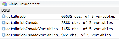
## 6 4 124 2012 106 NA## [1] 972 5The final dataset (dataUnidoCanadaVariablesAfter2009) is a dataframe of 972 rows and 5 columns. With the filter() function from the dplyr package, you can now manipule any dataset in order to filter and create a subset of it, based on any variable. In the following picture, you can see that each dataset is smaller and smaller than the previous one (these data are located in your environment panel).
To familiarize yourself with these manipulations, consider the following exercices:
Exercice 1: from the UNIDO database, create a dataframe concerning the number of employees in Canada; from 2009 to 2012
[Code]
library(gsheet)
library(dplyr)
dataUnido_ex1 <- gsheet2tbl("https://docs.google.com/spreadsheets/d/1uLaXke-KPN28-ESPPoihk8TiXVWp5xuNGHW7w7yqLCc/edit#gid=416085055")
dataUnido_ex1 <- rename(dataUnido_ex1, Country=countryCode)
dataUnido_ex1 <- rename(dataUnido_ex1, Year=year)
dataUnido_ex1 <- rename(dataUnido_ex1, Employees=tableDefinitionCode)
dataUnido_ex1[,8:10]<-NULL
dataUnido_ex1$tableCode<-NULL
dataUnido_ex1$isicCode<-NULL
dataUnido_ex1$isicCodeCombinaison<-NULL
dataUnido_ex1 <- filter(dataUnido_ex1, Country==124 & Year >=2009 & Year<=2012 & Employees == 04)
dataUnido_ex1Exercice 2: from the UNIDO database, create a dataframe concerning Dairy products from all country in 2011
[Code]
library(gsheet)
library(dplyr)
dataUnido_ex2 <- gsheet2tbl("https://docs.google.com/spreadsheets/d/1uLaXke-KPN28-ESPPoihk8TiXVWp5xuNGHW7w7yqLCc/edit#gid=416085055")
dataUnido_ex2 <- rename(dataUnido_ex2, Country=countryCode)
dataUnido_ex2 <- rename(dataUnido_ex2, Year=year)
dataUnido_ex2 <- rename(dataUnido_ex2, Employees=tableDefinitionCode)
dataUnido_ex2[,8:10] <- NULL
dataUnido_ex2$tableCode <- NULL
dataUnido_ex2$isicCodeCombinaison <- NULL
dataUnido_ex2 <- filter(dataUnido_ex2, isicCode==1520 & Year==2011 & Employees == 04)
dataUnido_ex2 <- arrange(dataUnido_ex2, desc(value))
dataUnido_ex27.4 Sorting data
At the present moment, your dataframe is sort by alphabetical order. By using the arrange() function of the dplyr package, it is possible to sort your dataframe depending on a variable. This can be done in ascending order or in descending order.
# dataSorted will receive the dataframe dataUnidoCanadaVariablesAfter2009 sorted by the column value
dataSorted <- arrange(dataUnidoCanadaVariablesAfter2009, value)
# dataReverse is the opposite of dataSorted, i.e. the first lines will have the highest values
dataReverse <- arrange(dataUnidoCanadaVariablesAfter2009, desc(value))We can compare both dataframes (dataSorted and dataReverse) to observe that they are arrange in different orders.
## # A tibble: 6 x 5
## tableCode countryCode year isicCode value
## <dbl> <dbl> <dbl> <dbl> <dbl>
## 1 1 124 2012 1072 8
## 2 1 124 2011 1072 15
## 3 1 124 2011 2814 18
## 4 1 124 2010 1200 19
## 5 1 124 2010 2814 19
## 6 1 124 2012 2814 19## # A tibble: 6 x 5
## tableCode countryCode year isicCode value
## <dbl> <dbl> <dbl> <dbl> <dbl>
## 1 4 124 2012 NA 1521817
## 2 4 124 2011 NA 1493703
## 3 4 124 2010 NA 1479914
## 4 4 124 2012 259 146628
## 5 4 124 2011 259 137810
## 6 4 124 2010 259 124923TL;DR
# Loading the gsheet package
library(gsheet)
# Read data from the URL
dataUnido <- gsheet::gsheet2tbl("https://docs.google.com/spreadsheets/d/1uLaXke-KPN28-ESPPoihk8TiXVWp5xuNGHW7w7yqLCc/edit#gid=416085055")
dataUnido
# Add a new column called 'newColumn'
dataUnido$newColumn <- 42

# Show the columns' name
colnames(dataUnido)
# Show the column 'newColumn'
dataUnido[,"newColumn"]
# Multiply by 2 and add 5
dataUnido$newColumn <- dataUnido$newColumn * 2 + 5

# Show the column 'newColumn'
dataUnido[,"newColumn"]
# Delete the column named 'newColumn'
dataUnido$newColumn <- NULL
# Show columns' name
colnames(dataUnido)
# erasing non important variables
dataUnido$isicCodeCombinaison <- NULL
dataUnido$tableDefinitionCode <- NULL
dataUnido$sourceCode <- NULL
dataUnido$updateYear <- NULL
dataUnido$unit <- NULL
# Provide first 6 lines of the dataframe
head(dataUnido)
# Provide the dimension of the dataframe
dim(dataUnido)
# Loading the dplyr package
library(dplyr)

# Subset of dataUnido based on countryCode == Canada
dataUnidoCanada <- filter(dataUnido, countryCode == 124)

# First lines of the dataframe
head(dataUnidoCanada)
# Number of columns & rows
dim(dataUnidoCanada)
# Subset of dataUnidoCanada based on two variables (number of employees and establishments)
dataUnidoCanadaVariables <- filter(dataUnidoCanada, tableCode == 4 | tableCode == 1)

# First lines of the dataframe
head(dataUnidoCanadaVariables)
# Last lines of the dataframe
tail(dataUnidoCanadaVariables)
# Number of columns & rows
dim(dataUnidoCanadaVariables)
# Subset of dataUnido based on countryCode == Canada
dataUnidoCanadaVariablesAfter2009 <- filter(dataUnidoCanadaVariables, year > 2009)

# First lines of the dataframe
head(dataUnidoCanadaVariablesAfter2009)
# Dimension of the dataframe
dim(dataUnidoCanadaVariablesAfter2009)
# dataSorted will receive the dataframe dataUnidoCanadaVariablesAfter2009 sorted by the column value
dataSorted <- arrange(dataUnidoCanadaVariablesAfter2009, value)

# dataReverse is the opposite of dataSorted, i.e. the first lines will have the highest values
dataReverse <- arrange(dataUnidoCanadaVariablesAfter2009, desc(value))
# first 6 lines of each dataset
head(dataSorted)
head(dataReverse)Code learned in this chapter
| Command | Detail |
|---|---|
| gsheet2tbl() | Download a table |
| colnames() | Retrieve or set the row or column names |
| head() | Returns the first rows |
| tail() | Returns the last rows |
| dim() | Retrieve or set the dimension of an object |
| arrange() | Sort rows in ascending order |
| desc() | Sort rows in descending order |
Getting your hands dirty
It’s time to practice! This exercise begins in Chapter 6 and continues through Chapter 9. This exercise is therefore divided into 4 parts. For this exercise, you’ll work with a csv file available on Github in the chapter6 folder.
Before starting the second part of this exercise, remember the first part:
- Step 1 : Import via a csv
Import the csv file called chapter6data.csv.
- Step 2 : Import via a gsheet
Import a dataset containing longitude and latitude from this gsheet: https://docs.google.com/spreadsheets/d/1nehKEBKTQx11LZuo5ZJFKTVS0p5y1ysMPSOSX_m8dS8/edit?usp=sharing
Now, let’s begin with the second part of this exercise:
- Step 3 : Delete the column
Delete the column X1.
- Step 4 : Filter the data
Filter the data to only keep the following countries: “United States”, “Canada”, “Japan”, “Belgium” and “France”.