Introduction
In this first chapter, you will familiarize yourself with the environment used in this book: RStudio.
What is it so unique about RStudio? Well, it is “just” another IDE (Integrated Development Environment). An IDE is nothing more than a graphical interface that connects a mouse click to a bash command or something not too far from that. So what is so great about RStudio? Well, they manged to put in one place, in a very fluid and integrated way, various languages such as R, Python and Markdown (to cite just a few). From there, you can write a business analyst report (that is the goal here) with Markdown and R. You could do it with Markdown and Python or Markdown and Julia likewise. Even if you are a true bash guy, the more you use RStudio, the more you realize how helpful it is too lower the barriers to entry to the programming world and power. I really believe they are among the players that truly help new generations to participate and take ownership of this industrial revolution 4.0.
This book is also a “hands-on” book. It will make you click and enter commands in your RStudio session to experience first-hand the process. Here, we stop before data modeling. Our aim here is to make students understand the concept and process of a data pipeline, from entering data into a data frame (something that looks like a Microsoft Excel sheet) to organizing and visualizing the data on a graph or in a series of graphs organized in a business dashboard.
The various examples will often be based on my research and the various datasets I have collected through time. All research projects presented here are made with RStudio, using the R programming language as well as Markdown.
The goal of this book is to harness the power of data science tools for business. In this regard, we promote reproducible research as our research method. In order to do so, RStudio, with documents written in Markdown, will be your main portal for doing your projects. You will learn a few syntax tips regarding Markdown and how to save your projects online (Git). Throughout the chapters, useful tips will be either displayed in bold or in italics.
At the end of the chapter, you should be able to:
- understand what an IDE is
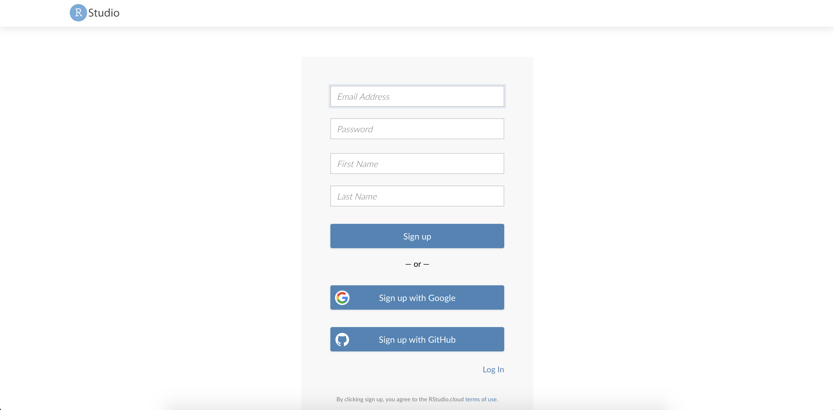
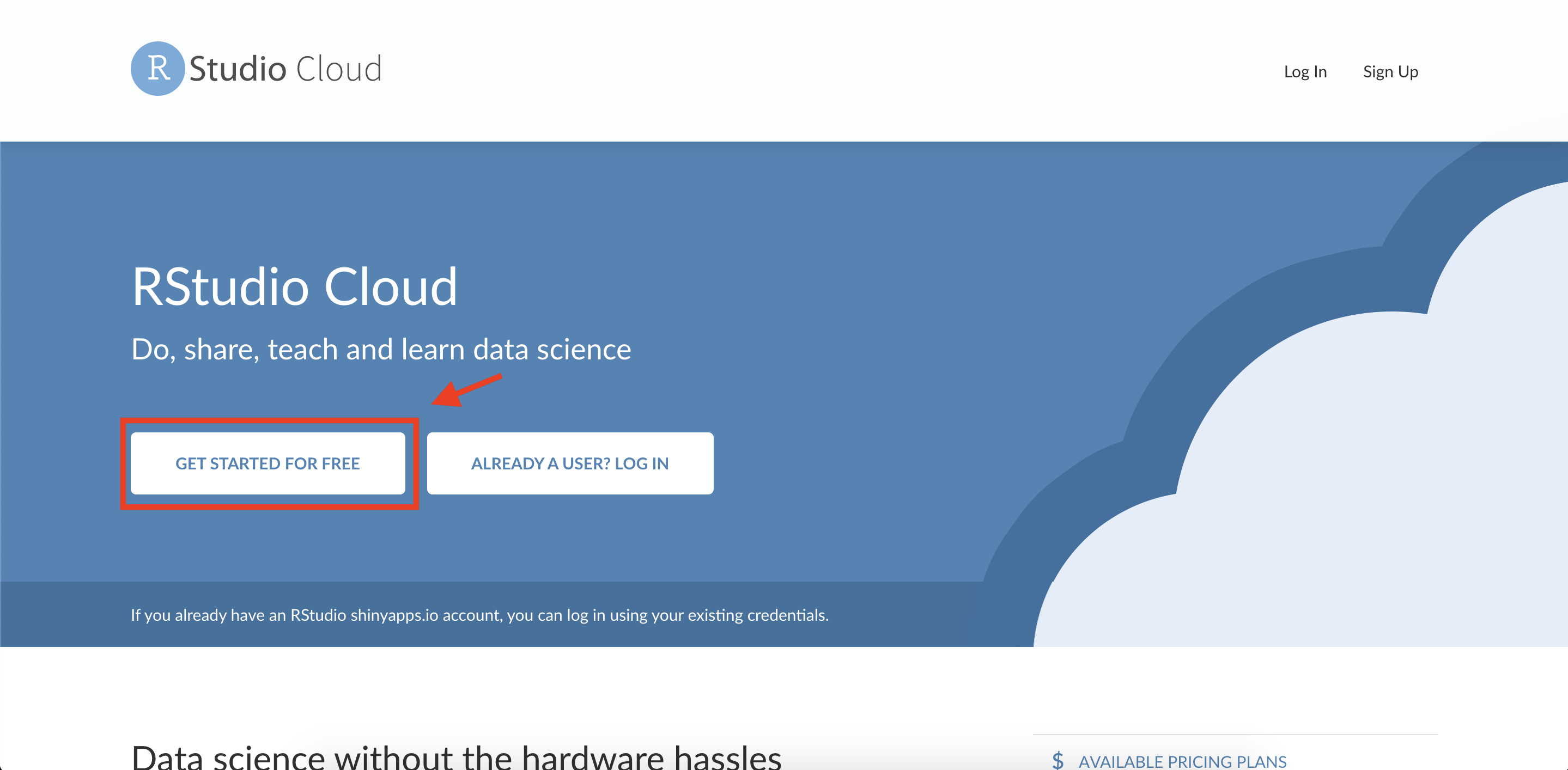
- create an account on Rstudio Cloud
- familiarize with the RStudio Integrated Development Environment
Environment
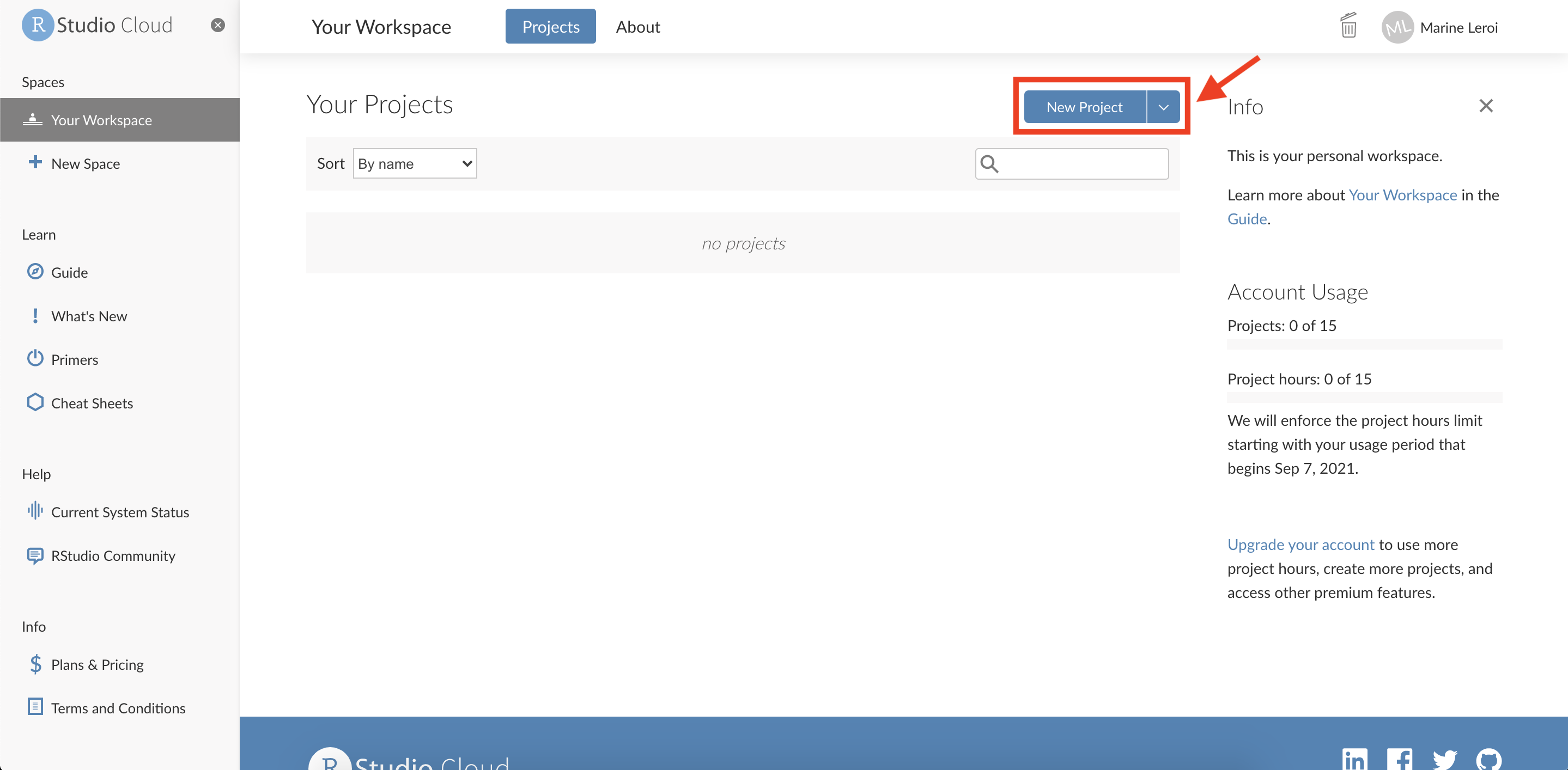
Now that you have created your account on RStudio.cloud, let’s begin with the environment.
Think about RStudio as Microsoft Office, the whole suite. Here, in the same interface you will be able to write text as you would do in Microsoft Word while being able to integrate some powerful commands in the same Word-style document. It is like having Excel embedded in Word, all in the same place. Even more than that, it is a super computer integrated in Word. It is indeed being able to leverage a great deal of computing power in something as easy to manipulate as Word. It is also live content. This is indeed the nature of coding. Every time you work on your document, the code runs as if it was the first time. It thus goes get the latest data available at the time you work on your document. It is always up-to-date.
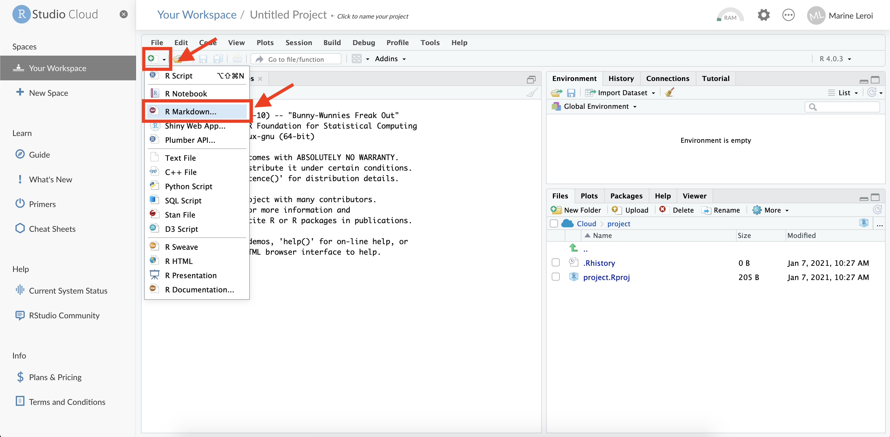
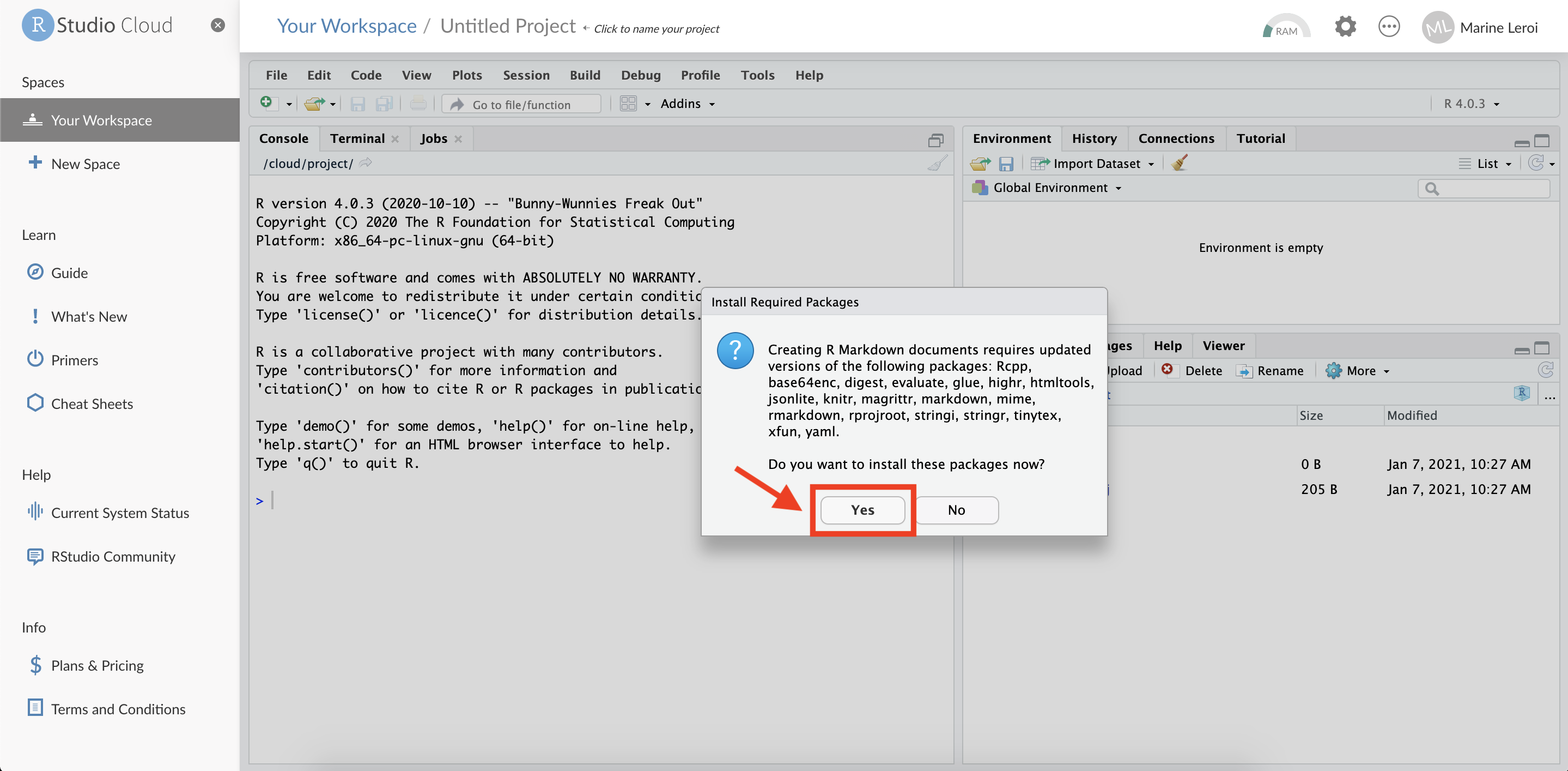
To really grasp what is happening, you need to get your hands dirty and go through the following steps. think that to “see” your final document, you will need to “compile” it. In order to do so, you will have to click on the “knit” button. That’s it.
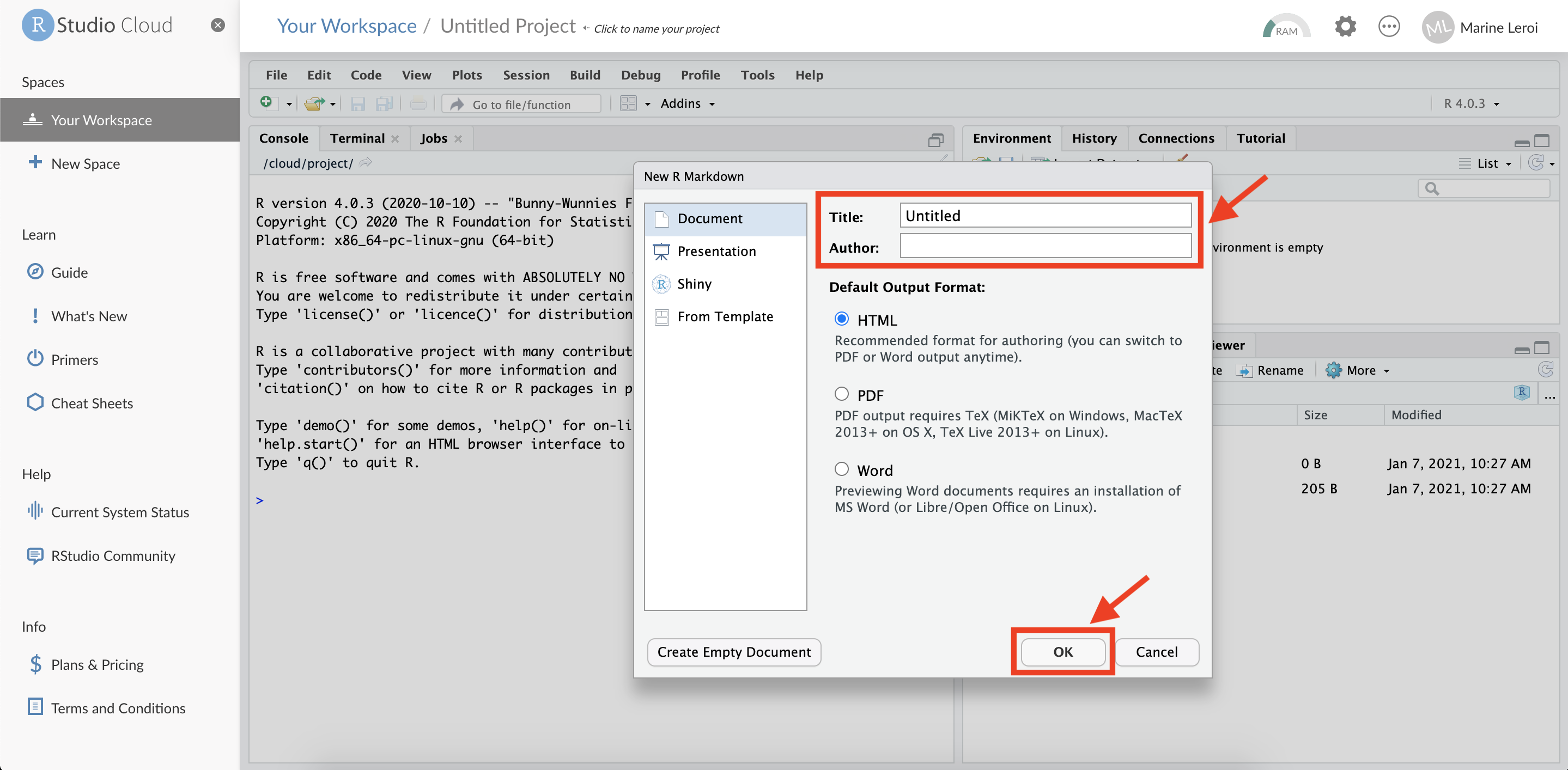
We will come back on that later, but the main difference with a Word document is its structure and in particular the top part of a document that we call “yaml.” Think about the yaml as the palce where you tell your computer how you want your document to be organized: what is the title, who is the author, what is the abstract, what is the output format (pdf, ppt), etc. Then, when you knit, your computer will take the information from this yaml and will just execute your orders.
This yaml is incredibly convenient, and also sometimes frustrating for Wrod users. It is incredibly convenient and fast because you can indicate that you want a pdf document and your report becomes a beautifully organized pdf document with a table of content, etc. If you wanted to generate a PPT with the same document, you change the output in the yaml, make some quick changes in your document, and you get a beautifully laid-out presentation. You just saved a lot of time. We all have spent a lot of time copying and pasting from Word to Powerpoint and being frustrated with the final result anyway because the images are not centered, etc. Here, the yaml takes care of that. Moreover, a year later, when you come back to this document, it will “knit” with the latest data, etc. Pretty cool.
Now it is frustrating for Word or Powerpoint users because they will not be able (or at least easily) to make all the changes they like, for instance changing the font size here and there, changing the colors, the location, etc. I know. the yaml can do tht but you need to be fluent in CSS. The good news is that you have a lot of templates in CSS for you. but my silver bullet to my students is to tell them that creating a beautiful document requires skills. It is a real job. Infographists know which font with which size, which color and which location work. I do not. So, Word or Powerpoint give me this freedom, but it is a freedom to very likely upset the professional eyes. Of course, my amateur friends may find that it looks good, but I want to appeal to a professional audience, not so much my friends. Okay, I stop here. I made my point.
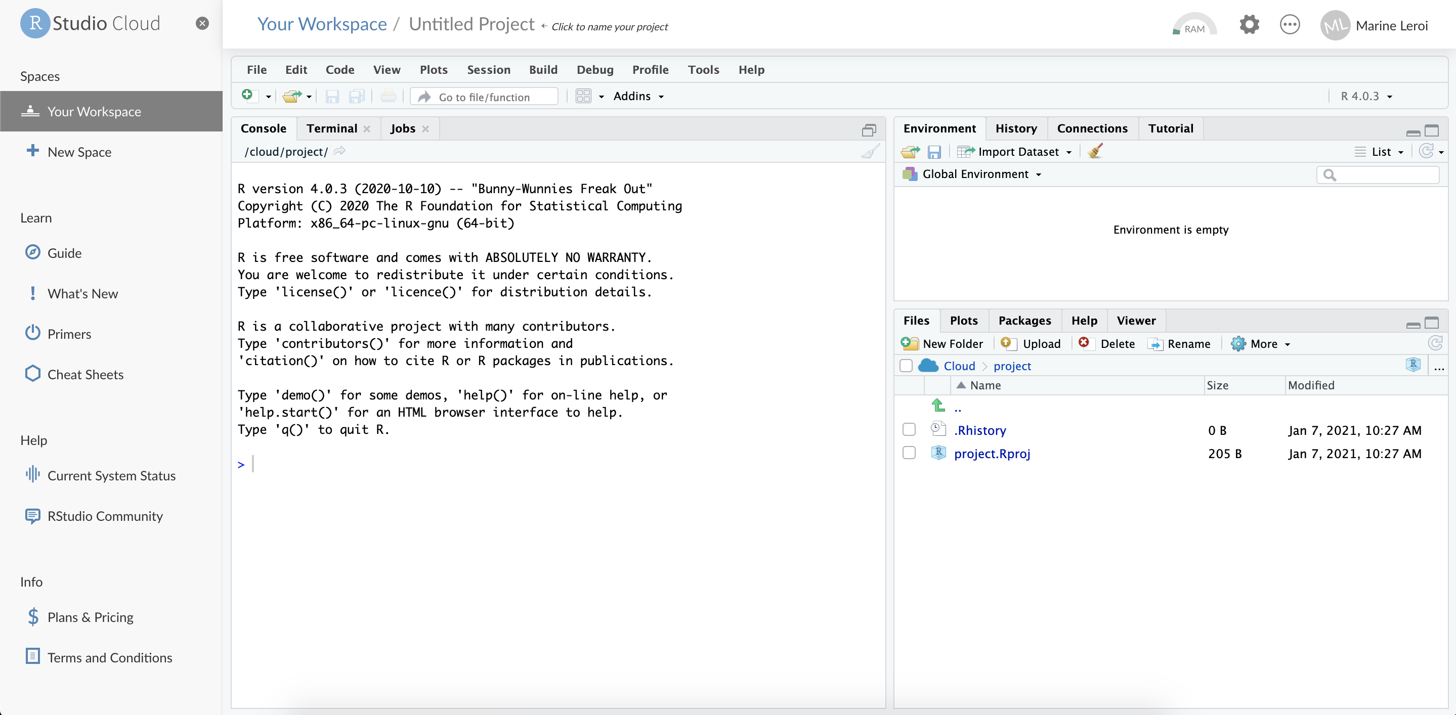
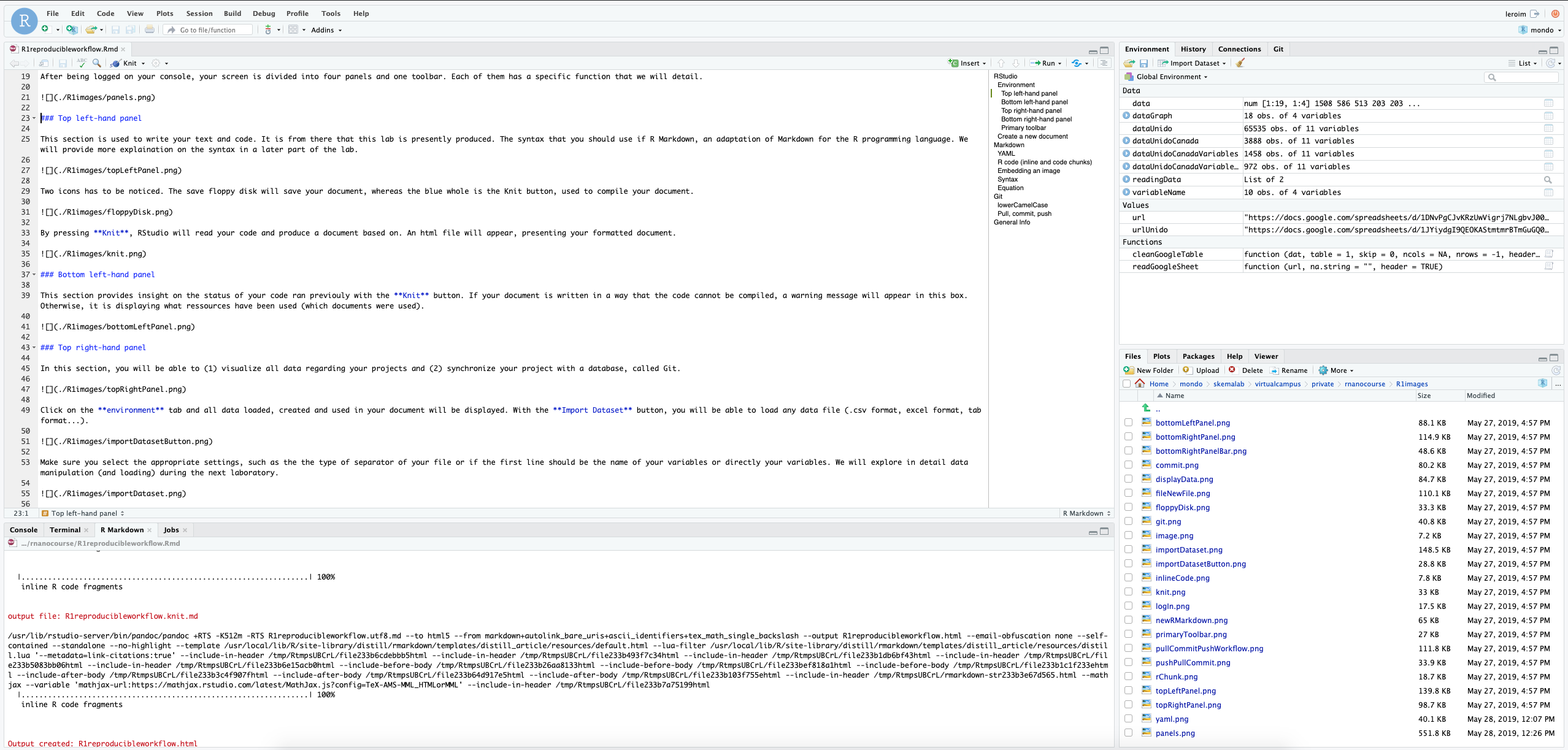
Let’s go now. After being logged on your console, your screen is divided into four panels and one toolbar. Each of them has a specific function that we will detail.
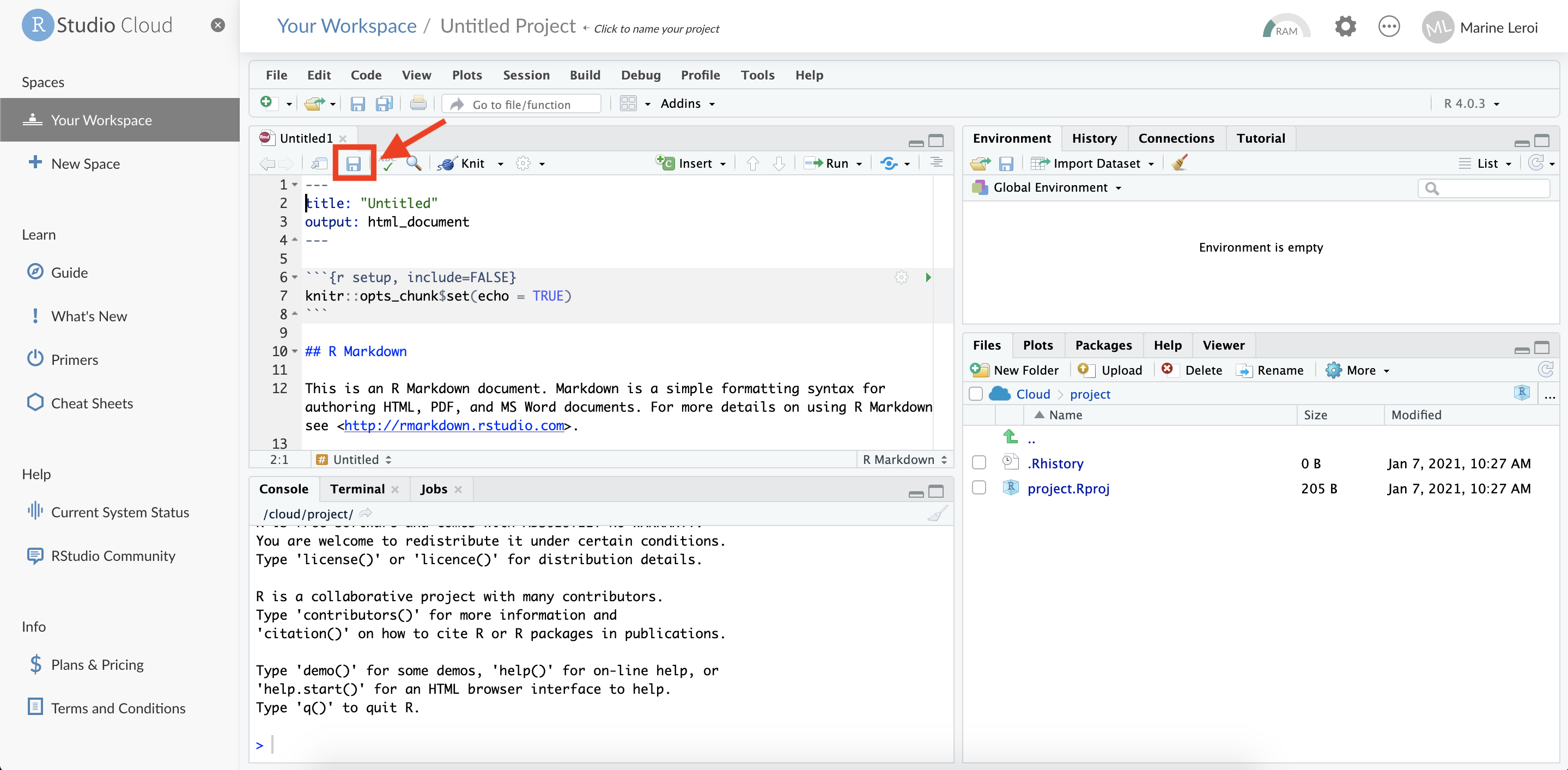
Top left-hand panel
This section is used to write your text and code. It is from there that this book is presently produced. The syntax that you should use is R Markdown, an adaptation of Markdown for the R programming language. We will provide more explanation on the syntax in the next chapter.
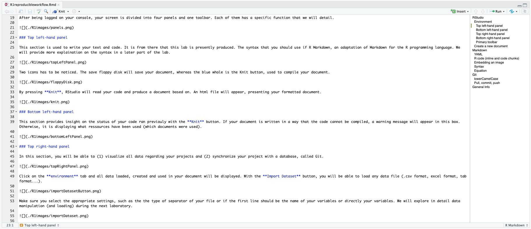
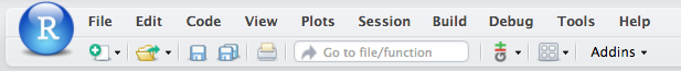
Two icons has to be noticed. The save floppy disk will save your document, whereas the blue whole is the Knit button, used to compile your document.

By pressing Knit, RStudio will read your code and produce a document. An html file will appear, presenting your formatted document.

By pressing the Document Outline icon, RStudio will show or hide the table of contents of your document.

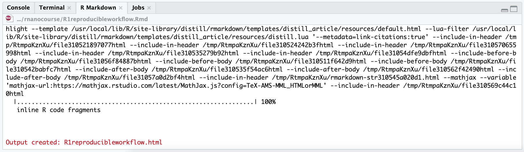
Bottom left-hand panel
This section provides an insight on the status of your code ran previously with the Knit button. If your document is written in a way that the code cannot be compiled, a warning message will appear in this box. Otherwise, it will display the resources (documents) that have been used.
Top right-hand panel
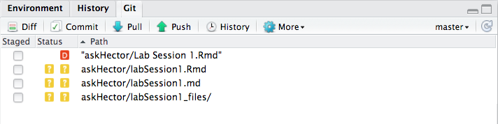
In this section, you will be able to (1) visualize all data regarding your projects and (2) synchronize your project with a database, called Git.
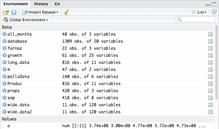
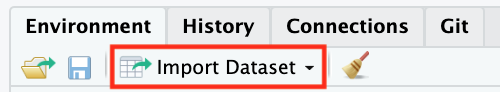
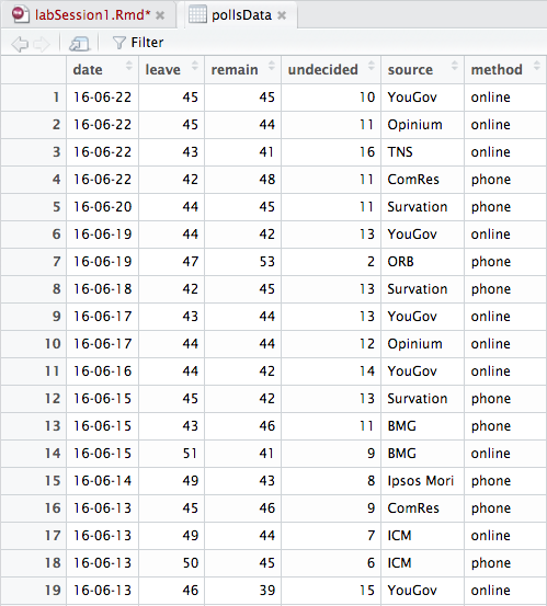
Click on the environment tab and all data loaded, created and used in your document will be displayed. With the Import Dataset button, you will be able to load any data file (.csv format, excel format, tab format…).
Make sure you select the appropriate settings, such as the the type of separator of your file or if the first line should be the name of your variables or directly your variables. We will explore in detail in the data wrangling chapters.
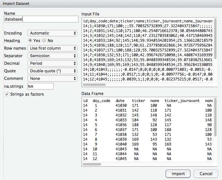
If you click on a specific data in the environment, the first 1,000 lines of data will be displayed.
Click on the Git tab and you may see a list of files. We will describe in details how to properly use the Git in order to synchronize your project on an online database.
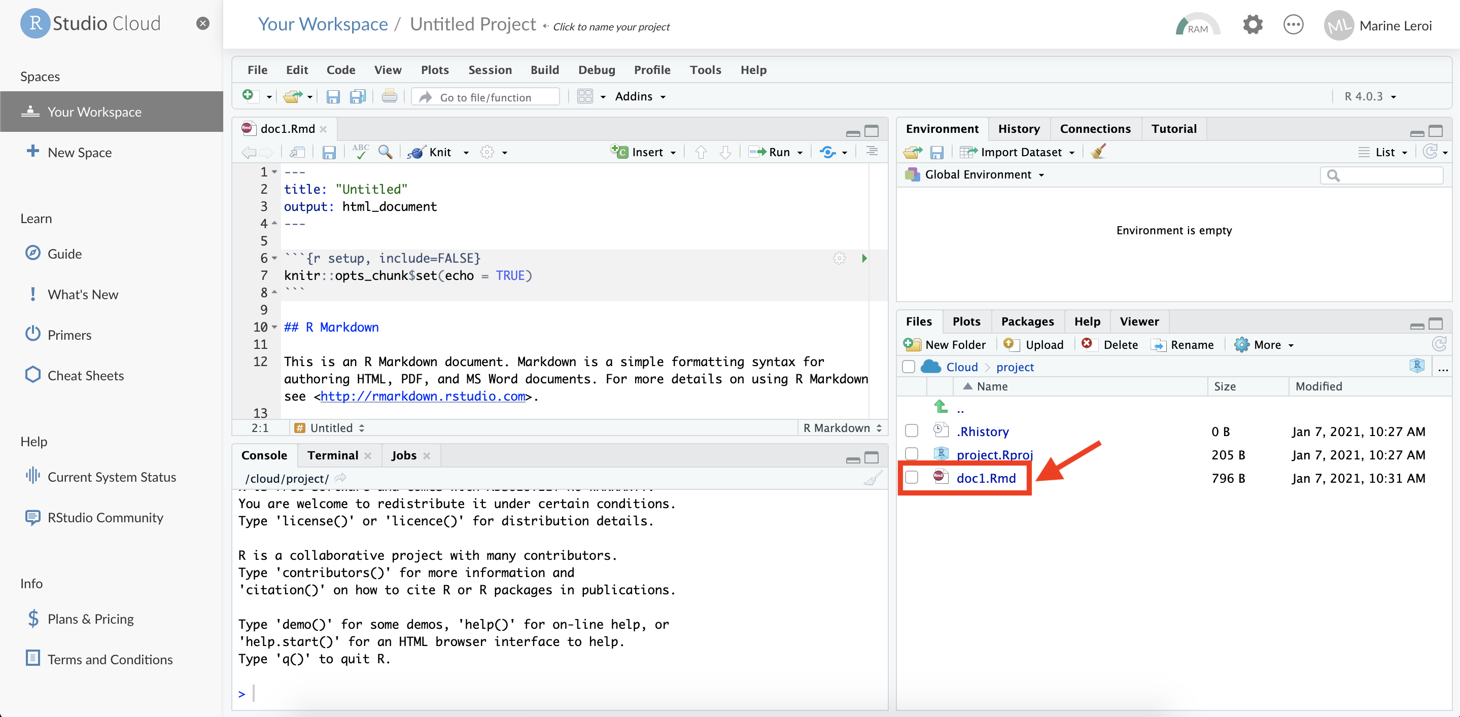
Bottom right-hand panel
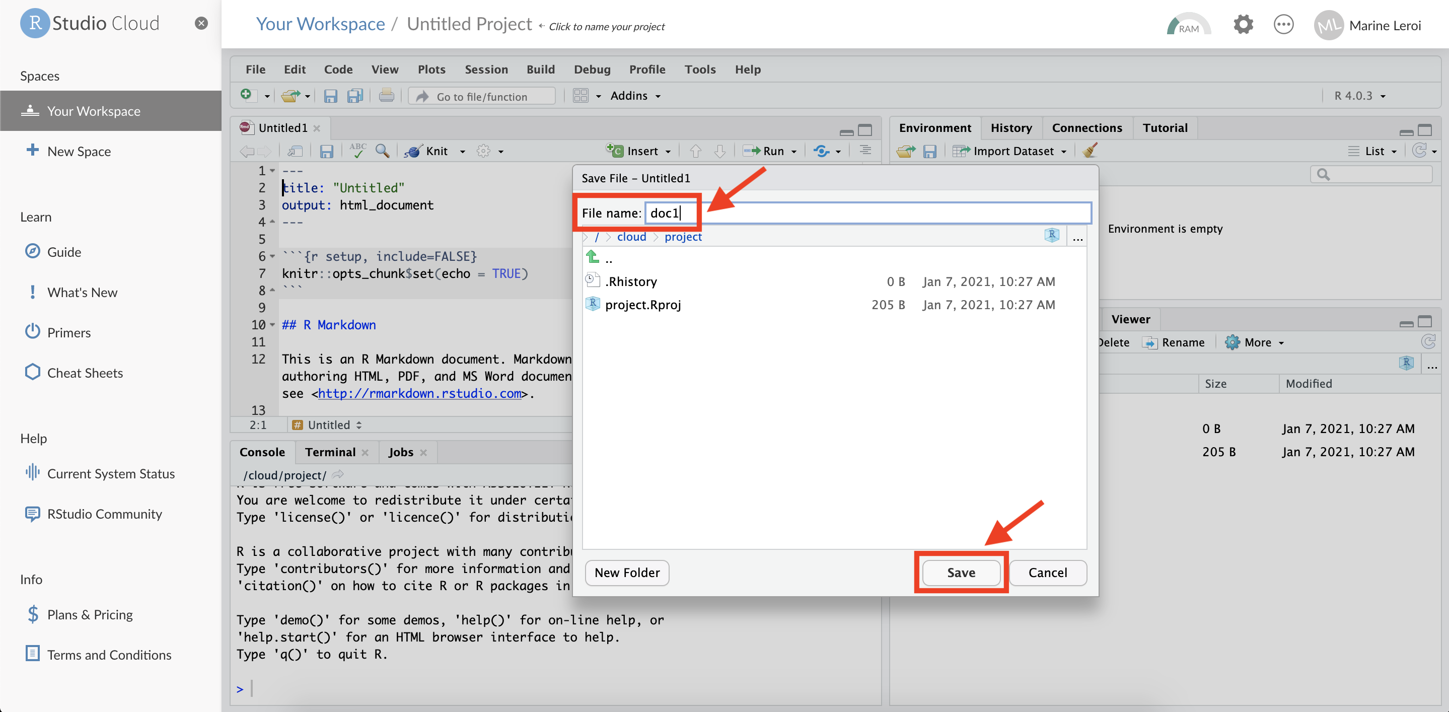
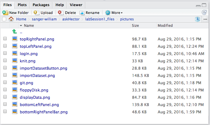
In the last panel, you will find all files available in your project under the Files tab. Note the path to reach each file, which may be useful when linking a picture or a dataset to the document your are editing. For example, the next picture will have a specific path, i.e.: ./R1images/bottomRightPanel.png. This indicates that the picture called bottomRightPanel.png is located in the pictures folder which in turn is in the labR1_files folder.
Think of this window as your finder on MacOs or file explorer on Windows machines.
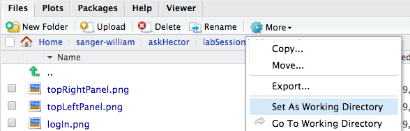
You can create a new folder by clicking on the New Folder button or change any setting of any file with the subsequent buttons. After clicking on the More button (blue engine), you will find the option to export any selected file. The option Set As Working Directory will indicate to RStudio from which file you are working from (in all the previous picture imports, the working directory was askHector, hence the ./ before each picture path details on how to use the Markdown syntax are provided in the next part).
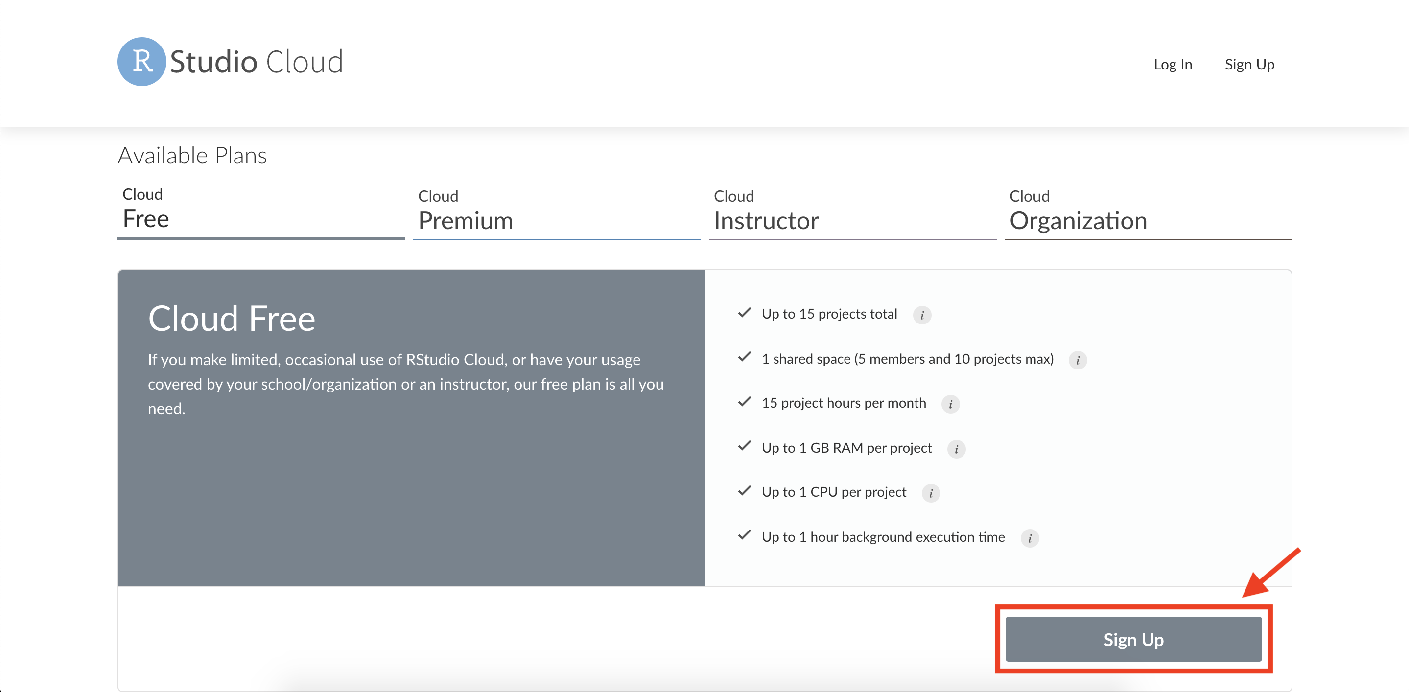 4. Choose which way you want to sign up.