Chapter 2 Markdown
2.1 Introduction
In this first chapter, you will familiarize yourself with one of the two main languages we will use in this book: Markdown. The other one being R.
Remember, the goal of this book is to harness the power of data science tools for business. In this regard, we promote reproducible research as our research method. In order to do so, RStudio, with documents written in Markdown, will be your main portal for doing your projects. You will learn a few syntax tips regarding Markdown and how to save your projects online (Git). Throughout the chapters, useful tips will be either displayed in bold or in italics.
At the end of the chapter, you should be able to:
- create your first document in RStudio
- understand the Markdown syntax and knit your document
2.2 Create a new document
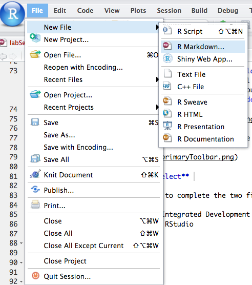
To create a new document, select File > New File > R Markdown.
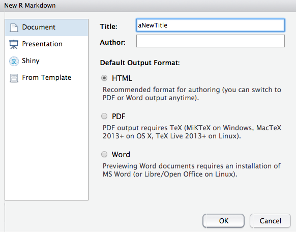
Select Document and enter the name of your new file with the default output format as HTML.
This will create a new file that you will be able to work with using the R Markdown syntax. Save your new file using the floppy disk icon seen previously.
At this point, you should be able to complete the two first achievements of the lab, namely:
- familiarize yourself with the RStudio Integrated Development Environment
- create your first document in RStudio
2.3 Markdown
Your newly created document will be written using the Markdown syntax. Such format incorporates R code (named chunks), provides the possibility to write mathematical equations in LaTeX and export your document to any format (presentation, html, .doc, PDF…).
For more on R Markdown syntax, please refer to: https://www.rstudio.com/wp-content/uploads/2015/02/rmarkdown-cheatsheet.pdf
2.3.1 YAML
At the beggining of the document lies the YAML, which dictates how the document will be formatted. The following lines of codes enables to write the author’s name, the date and the desired output (here an html document with a table of content).
You can change the desired output by selecting a specific option:
- output: html_document -> html file
- output: pdf_document -> PDF
- output: word_document -> .docx document
- output: bearmer_presentation -> powerpoint-like presentation
- output: ioslides_presentation -> powerpoint-like presentation (html format)
- output: github_document -> format for GitHub
2.3.2 R code
We have a special chapter on the grammar of R and its terminology. For now, we will remain at a bird’s eye view.
2.3.2.1 Code Chunk
Reproducible research seeks to provide multiple analysis of a same dataset, and verify each result even thought data are changed during the process. Hence, by using R Markdown, it is possible to add R code, which are coding and programming parts to analyze data. In order to do so, you should write your R code in between 3 ticks called a R chunck, such as:
The first line will provide some descriptive statistics of a dataset (here named cars).
Whereas the second line of code will plot a graph of the previous data.
You should notice that a comment in a R chunck is written with a # before the beginning of the sentence.
2.3.2.2 Inline Code
For inline coding, instead of 3 ticks, a single tick with r is required, such as:
This code generate the average speed. Integrated in a sentence it looks like this:
The result: The average speed of the dataset is equal to 15.4 mile per hour.
2.3.3 Embedding an image
Insert an image into your document by writting the following ponctuations: exclamation mark, brackets, parenthesis, with the path of the image inside parenthesis. For example:
2.3.4 Syntax
R Markdown has specific formatting settings that will be understood by RStudio.
- For bold text, encapsulate the text in between 2 stars. A bold text;
- For italic text, encapsulate the text in between 1 star. An italic text;
- For superscript text, encapsulate the text in between 1 circumflex.superscript;
- For linking a webpage to a text, provide the link with the following syntax: brackets parenthesis, with the link inside parenthesis and your text inside brackets. Link to www.warin.ca.
A title has to be specified by a hash character (#). The number of # indicated the level of title: for example a second-order title will be preceded by ##, whereas a third level title will be preceded by ### (you have multiple examples in the present document).
2.3.5 Equation
Finally, you can write any equation using the LaTeX format in R Markdown. In order to do so, you have to insert your equation in a LaTeX format between two $.
For example, this equation:
Will generate this:
\(y_i= \alpha_0 + \alpha_1.x_1+\alpha_2.x_2+\alpha_3.x_3+\epsilon\)
By this point, you should be able to complete the third achievement of the chapter, namely:
- understand the Markdown syntax and knit your document
2.4 Reproducible research
In this book, we like reproducible research a lot! It allows people across the world to have access to the explanations through an article, the code and the data. By sharing all this information, we all save a lot of time and can all move further in the various developments.
Here is a fantastic Shiny app with references of economic articles accompanied by their code and data. It is very useful to select an article for an individual project or for a team project in a course.
Economic articles - reproducible research
TL;DR
---
title: "aNewTitle"
author: "John Doe"
date: "28/05/2019"
output: html_document
---
# provide some descriptive statistics
summary(cars)
# plot a 2 axis graph
plot(cars)
# inline code
`r mean(cars$speed)`
# set up images
Code learned in this chapter
| Command | Detail |
|---|---|
| summary() | Produce result summaries |
| plot() | Plot of R objects |
| mean() | Calculate (trimmed) arithmetic mean |
Getting your hands dirty
To get familiar with Markdown, you must reproduce this report. A copy and images are also available in folder named chapter2 on Github. It needs to be perfectly identical. Make sure that you respect the different levels of headings and the typography. Do not forget to add images and the html link.
We recommend you to review this chapter and consult the R Markdown Cheat Sheet